Heat equation - Mixed H(div) conforming formulation)

As an alternative to the standard formulation for solving the heat equation used in the heat equation tutorial, we can used a mixed formulation where both the temperature, $u(\mathbf{x})$, and the heat flux, $\boldsymbol{q}(\boldsymbol{x})$, are primary variables. From a theoretical standpoint, there are many details on e.g. which combinations of interpolations that are stable. See e.g. [1] and [2] for further reading. This tutorial is based on the theory in FEniCSx' mixed poisson example.

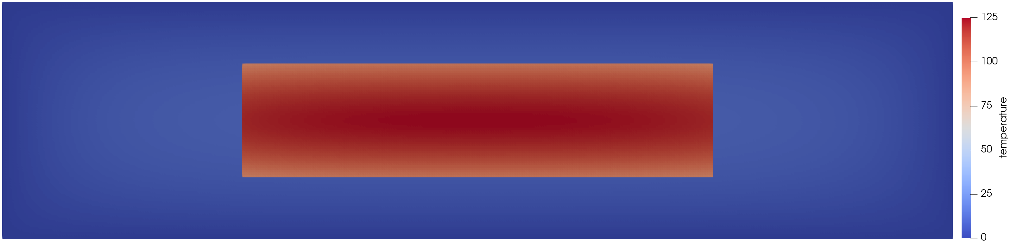Figure: Temperature distribution considering a central part with lower heat conductivity.

The advantage with the mixed formulation is that the heat flux is approximated better. However, the temperature becomes discontinuous where the conductivity is discontinuous.

Theory

We start with the strong form of the heat equation: Find the temperature, $u(\boldsymbol{x})$, and heat flux, $\boldsymbol{q}(x)$, such that

\[\begin{align*} \boldsymbol{\nabla}\cdot \boldsymbol{q} &= h(\boldsymbol{x}), \quad \text{in } \Omega \\ \boldsymbol{q}(\boldsymbol{x}) &= - k\ \boldsymbol{\nabla} u(\boldsymbol{x}), \quad \text{in } \Omega \\ \boldsymbol{q}(\boldsymbol{x})\cdot \boldsymbol{n}(\boldsymbol{x}) &= q_n, \quad \text{on } \Gamma_\mathrm{N}\\ u(\boldsymbol{x}) &= u_\mathrm{D}, \quad \text{on } \Gamma_\mathrm{D} \end{align*}\]

From this strong form, we can formulate the weak form as a mixed formulation. Find $u \in \mathbb{U}$ and $\boldsymbol{q}\in\mathbb{Q}$ such that

\[\begin{align*} \int_{\Omega} \delta u [\boldsymbol{\nabla} \cdot \boldsymbol{q}]\ \mathrm{d}\Omega &= \int_\Omega \delta u h\ \mathrm{d}\Omega, \quad \forall\ \delta u \in \delta\mathbb{U} \\ % \int_{\Omega} \boldsymbol{\delta q} \cdot \boldsymbol{q}\ \mathrm{d}\Omega &= -\int_\Omega \boldsymbol{\delta q} \cdot [k\ \boldsymbol{\nabla} u]\ \mathrm{d}\Omega \\ \int_{\Omega} \boldsymbol{\delta q} \cdot \boldsymbol{q}\ \mathrm{d}\Omega - \int_{\Omega} [\boldsymbol{\nabla} \cdot \boldsymbol{\delta q}] k u \ \mathrm{d}\Omega &= -\int_\Gamma \boldsymbol{\delta q} \cdot \boldsymbol{n} k\ u\ \mathrm{d}\Gamma, \quad \forall\ \boldsymbol{\delta q} \in \delta\mathbb{Q} \end{align*}\]

where we have the function spaces,

\[\begin{align*} \mathbb{U} &= \delta\mathbb{U} = L^2 \\ \mathbb{Q} &= \lbrace \boldsymbol{q} \in H(\mathrm{div}) \text{ such that } \boldsymbol{q}\cdot\boldsymbol{n} = q_\mathrm{n} \text{ on } \Gamma_\mathrm{D}\rbrace \\ \delta\mathbb{Q} &= \lbrace \boldsymbol{q} \in H(\mathrm{div}) \text{ such that } \boldsymbol{q}\cdot\boldsymbol{n} = 0 \text{ on } \Gamma_\mathrm{D}\rbrace \end{align*}\]

A stable choice of finite element spaces for this problem on grid with triangles is using

• DiscontinuousLagrange{RefTriangle, k-1} for approximating $L^2$
• BrezziDouglasMarini{RefTriangle, k} for approximating $H(\mathrm{div})$

Dirichlet BC theory for hdiv interpolations.

For a field representing a flux, we in general set the boundary condition on the normal component of this flux. Consider the field $\boldsymbol{q}(\boldsymbol{x})$, then we want to prescribe $q_\mathrm{n}(\boldsymbol{x}) = \boldsymbol{q}(\boldsymbol{x}) \cdot \boldsymbol{n}$, which we can calculate as

\[q_\mathrm{n}(\boldsymbol{x}) = [\boldsymbol{N}_i(\boldsymbol{x}) \cdot \boldsymbol{n}] a_i\]

However, for $H(\mathrm{div})$ interpolations, we don't have distinct algebraic nodal coordinates, $\boldsymbol{x}_j$, fulfilling $\vert\boldsymbol{N}_i(\boldsymbol{x}_j)\vert = \delta_{ij}$. Instead, we have

\[\begin{align*} \int_0^1 s (4-6s) \mathrm{d}s = [2s^2 - 2 s^3] = 0\\ \int_0^1 (1-s) (4-6s) \mathrm{d}s = \int_0^1 4 - 10s + 6s^2 \mathrm{d}s = [4s - 5s^2 + 2s^3] = 1 \end{align*}\]

Commented Program

Now we solve the problem in Ferrite. What follows is a program spliced with comments.

First we load Ferrite,

using Ferrite

And define our grid, representing a channel with a central part having a lower conductivity, $k$, than the surrounding.

function create_grid(ny::Int)
    width = 10.0
    length = 40.0
    center_width = 5.0
    center_length = 20.0
    upper_right = Vec((length / 2, width / 2))
    grid = generate_grid(Triangle, (round(Int, ny * length / width), ny), -upper_right, upper_right)
    addcellset!(grid, "center", x -> abs(x[1]) < center_length / 2 && abs(x[2]) < center_width / 2)
    addcellset!(grid, "around", setdiff(1:getncells(grid), getcellset(grid, "center")))
    return grid
end

grid = create_grid(10)

Setup

We define one CellValues for each field which share the same quadrature rule.

ip_geo = geometric_interpolation(getcelltype(grid))
ipu = DiscontinuousLagrange{RefTriangle, 0}()
ipq = BrezziDouglasMarini{2, RefTriangle, 1}()
qr = QuadratureRule{RefTriangle}(2)
cellvalues = (u = CellValues(qr, ipu, ip_geo), q = CellValues(qr, ipq, ip_geo))

Distribute the degrees of freedom

dh = DofHandler(grid)
add!(dh, :u, ipu)
add!(dh, :q, ipq)
close!(dh)

In this problem, we have a zero temperature on the boundary, Γ, which is enforced via zero Neumann boundary conditions. Hence, we don't need a Constrainthandler.

Γ = union((getfacetset(grid, name) for name in ("left", "right", "bottom", "top"))...)

Element implementation

function assemble_element!(Ke::Matrix, fe::Vector, cv::NamedTuple, dr::NamedTuple, k::Number)
    cvu = cv[:u]
    cvq = cv[:q]
    dru = dr[:u]
    drq = dr[:q]
    h = 1.0 # Heat source
    # Loop over quadrature points
    for q_point in 1:getnquadpoints(cvu)
        # Get the quadrature weight
        dΩ = getdetJdV(cvu, q_point)
        # Loop over test shape functions
        for (iu, Iu) in pairs(dru)
            δNu = shape_value(cvu, q_point, iu)
            # Add contribution to fe
            fe[Iu] += δNu * h * dΩ
            # Loop over trial shape functions
            for (jq, Jq) in pairs(drq)
                div_Nq = shape_divergence(cvq, q_point, jq)
                # Add contribution to Ke
                Ke[Iu, Jq] += (δNu * div_Nq) * dΩ
            end
        end
        for (iq, Iq) in pairs(drq)
            δNq = shape_value(cvq, q_point, iq)
            div_δNq = shape_divergence(cvq, q_point, iq)
            for (ju, Ju) in pairs(dru)
                Nu = shape_value(cvu, q_point, ju)
                Ke[Iq, Ju] -= div_δNq * k * Nu * dΩ
            end
            for (jq, Jq) in pairs(drq)
                Nq = shape_value(cvq, q_point, jq)
                Ke[Iq, Jq] += (δNq ⋅ Nq) * dΩ
            end
        end
    end
    return Ke, fe
end

Global assembly

function assemble_global(cellvalues, dh::DofHandler)
    grid = dh.grid
    # Allocate the element stiffness matrix and element force vector
    dofranges = (u = dof_range(dh, :u), q = dof_range(dh, :q))
    ncelldofs = ndofs_per_cell(dh)
    Ke = zeros(ncelldofs, ncelldofs)
    fe = zeros(ncelldofs)
    # Allocate global system matrix and vector
    K = allocate_matrix(dh)
    f = zeros(ndofs(dh))
    # Create an assembler
    assembler = start_assemble(K, f)
    x = copy(getcoordinates(grid, 1))
    dofs = copy(celldofs(dh, 1))
    # Loop over all cells
    for (cells, k) in (
            (getcellset(grid, "center"), 0.1),
            (getcellset(grid, "around"), 1.0),
        )
        for cellnr in cells
            # Reinitialize cellvalues for this cell
            cell = getcells(grid, cellnr)
            getcoordinates!(x, grid, cell)
            celldofs!(dofs, dh, cellnr)
            reinit!(cellvalues[:u], cell, x)
            reinit!(cellvalues[:q], cell, x)
            # Reset to 0
            fill!(Ke, 0)
            fill!(fe, 0)
            # Compute element contribution
            assemble_element!(Ke, fe, cellvalues, dofranges, k)
            # Assemble Ke and fe into K and f
            assemble!(assembler, dofs, Ke, fe)
        end
    end
    return K, f
end

Solution of the system

K, f = assemble_global(cellvalues, dh);
u = K \ f

Exporting to VTK

Currently, exporting discontinuous interpolations is not supported. Since in this case, we have a single temperature degree of freedom per cell, we work around this by calculating the per-cell temperature.

temperature_dof = first(dof_range(dh, :u))
u_cells = map(1:getncells(grid)) do i
    u[celldofs(dh, i)[temperature_dof]]
end
VTKGridFile("heat_equation_hdiv", dh) do vtk
    write_cell_data(vtk, u_cells, "temperature")
end

Postprocess the total flux

We applied a constant unit heat source to the body, and the total heat flux exiting across the boundary should therefore match the area for the considered stationary case.

function calculate_flux(dh, boundary_facets, ip, a)
    grid = dh.grid
    qr = FacetQuadratureRule{RefTriangle}(4)
    ip_geo = geometric_interpolation(getcelltype(grid))
    fv = FacetValues(qr, ip, ip_geo)

    dofrange = dof_range(dh, :q)
    flux = 0.0
    dofs = celldofs(dh, 1)
    ae = zeros(length(dofs))
    x = getcoordinates(grid, 1)
    for (cellnr, facetnr) in boundary_facets
        getcoordinates!(x, grid, cellnr)
        cell = getcells(grid, cellnr)
        celldofs!(dofs, dh, cellnr)
        map!(i -> a[i], ae, dofs)
        reinit!(fv, cell, x, facetnr)
        for q_point in 1:getnquadpoints(fv)
            dΓ = getdetJdV(fv, q_point)
            n = getnormal(fv, q_point)
            q = function_value(fv, q_point, ae, dofrange)
            flux += (q ⋅ n) * dΓ
        end
    end
    return flux
end

println("Outward flux: ", calculate_flux(dh, Γ, ipq, u))

Outward flux: 400.0000000000002

Note that this is not the case for the standard Heat equation, as the flux terms are less accurately approximated. A fine mesh is required to converge in that case. However, the present example gives a worse approximation of the temperature field.

Plain program

Here follows a version of the program without any comments. The file is also available here: heat_equation_hdiv.jl.

using Ferrite

function create_grid(ny::Int)
    width = 10.0
    length = 40.0
    center_width = 5.0
    center_length = 20.0
    upper_right = Vec((length / 2, width / 2))
    grid = generate_grid(Triangle, (round(Int, ny * length / width), ny), -upper_right, upper_right)
    addcellset!(grid, "center", x -> abs(x[1]) < center_length / 2 && abs(x[2]) < center_width / 2)
    addcellset!(grid, "around", setdiff(1:getncells(grid), getcellset(grid, "center")))
    return grid
end

grid = create_grid(10)

ip_geo = geometric_interpolation(getcelltype(grid))
ipu = DiscontinuousLagrange{RefTriangle, 0}()
ipq = BrezziDouglasMarini{2, RefTriangle, 1}()
qr = QuadratureRule{RefTriangle}(2)
cellvalues = (u = CellValues(qr, ipu, ip_geo), q = CellValues(qr, ipq, ip_geo))

dh = DofHandler(grid)
add!(dh, :u, ipu)
add!(dh, :q, ipq)
close!(dh)

Γ = union((getfacetset(grid, name) for name in ("left", "right", "bottom", "top"))...)

function assemble_element!(Ke::Matrix, fe::Vector, cv::NamedTuple, dr::NamedTuple, k::Number)
    cvu = cv[:u]
    cvq = cv[:q]
    dru = dr[:u]
    drq = dr[:q]
    h = 1.0 # Heat source
    # Loop over quadrature points
    for q_point in 1:getnquadpoints(cvu)
        # Get the quadrature weight
        dΩ = getdetJdV(cvu, q_point)
        # Loop over test shape functions
        for (iu, Iu) in pairs(dru)
            δNu = shape_value(cvu, q_point, iu)
            # Add contribution to fe
            fe[Iu] += δNu * h * dΩ
            # Loop over trial shape functions
            for (jq, Jq) in pairs(drq)
                div_Nq = shape_divergence(cvq, q_point, jq)
                # Add contribution to Ke
                Ke[Iu, Jq] += (δNu * div_Nq) * dΩ
            end
        end
        for (iq, Iq) in pairs(drq)
            δNq = shape_value(cvq, q_point, iq)
            div_δNq = shape_divergence(cvq, q_point, iq)
            for (ju, Ju) in pairs(dru)
                Nu = shape_value(cvu, q_point, ju)
                Ke[Iq, Ju] -= div_δNq * k * Nu * dΩ
            end
            for (jq, Jq) in pairs(drq)
                Nq = shape_value(cvq, q_point, jq)
                Ke[Iq, Jq] += (δNq ⋅ Nq) * dΩ
            end
        end
    end
    return Ke, fe
end

function assemble_global(cellvalues, dh::DofHandler)
    grid = dh.grid
    # Allocate the element stiffness matrix and element force vector
    dofranges = (u = dof_range(dh, :u), q = dof_range(dh, :q))
    ncelldofs = ndofs_per_cell(dh)
    Ke = zeros(ncelldofs, ncelldofs)
    fe = zeros(ncelldofs)
    # Allocate global system matrix and vector
    K = allocate_matrix(dh)
    f = zeros(ndofs(dh))
    # Create an assembler
    assembler = start_assemble(K, f)
    x = copy(getcoordinates(grid, 1))
    dofs = copy(celldofs(dh, 1))
    # Loop over all cells
    for (cells, k) in (
            (getcellset(grid, "center"), 0.1),
            (getcellset(grid, "around"), 1.0),
        )
        for cellnr in cells
            # Reinitialize cellvalues for this cell
            cell = getcells(grid, cellnr)
            getcoordinates!(x, grid, cell)
            celldofs!(dofs, dh, cellnr)
            reinit!(cellvalues[:u], cell, x)
            reinit!(cellvalues[:q], cell, x)
            # Reset to 0
            fill!(Ke, 0)
            fill!(fe, 0)
            # Compute element contribution
            assemble_element!(Ke, fe, cellvalues, dofranges, k)
            # Assemble Ke and fe into K and f
            assemble!(assembler, dofs, Ke, fe)
        end
    end
    return K, f
end

K, f = assemble_global(cellvalues, dh);
u = K \ f

temperature_dof = first(dof_range(dh, :u))
u_cells = map(1:getncells(grid)) do i
    u[celldofs(dh, i)[temperature_dof]]
end
VTKGridFile("heat_equation_hdiv", dh) do vtk
    write_cell_data(vtk, u_cells, "temperature")
end

function calculate_flux(dh, boundary_facets, ip, a)
    grid = dh.grid
    qr = FacetQuadratureRule{RefTriangle}(4)
    ip_geo = geometric_interpolation(getcelltype(grid))
    fv = FacetValues(qr, ip, ip_geo)

    dofrange = dof_range(dh, :q)
    flux = 0.0
    dofs = celldofs(dh, 1)
    ae = zeros(length(dofs))
    x = getcoordinates(grid, 1)
    for (cellnr, facetnr) in boundary_facets
        getcoordinates!(x, grid, cellnr)
        cell = getcells(grid, cellnr)
        celldofs!(dofs, dh, cellnr)
        map!(i -> a[i], ae, dofs)
        reinit!(fv, cell, x, facetnr)
        for q_point in 1:getnquadpoints(fv)
            dΓ = getdetJdV(fv, q_point)
            n = getnormal(fv, q_point)
            q = function_value(fv, q_point, ae, dofrange)
            flux += (q ⋅ n) * dΓ
        end
    end
    return flux
end

println("Outward flux: ", calculate_flux(dh, Γ, ipq, u))

This page was generated using Literate.jl.