Topology optimization

Keywords: Topology optimization, weak and strong form, non-linear problem, Laplacian, grid topology

Figure 1: Evolution of the material density during topology optimization of the bending beam for a fixed total mass.

Introduction

Topology optimization is the task of finding structures that are mechanically ideal. In this example we cover the bending beam, where we specify a load, boundary conditions and the total mass. Then, our objective is to find the most suitable geometry within the design space minimizing the compliance (i.e. the inverse stiffness) of the structure. We shortly introduce our simplified model for regular meshes. A detailed derivation of the method and advanced techniques can be found in [17] and [18].

We start by introducing the local, elementwise density $\chi \in [\chi_{\text{min}}, 1]$ of the material, where we choose $\chi_{\text{min}}$ slightly above zero to prevent numerical instabilities. Here, $\chi = \chi_{\text{min}}$ means void and $\chi=1$ means bulk material. Then, we use a SIMP ansatz (solid isotropic material with penalization) for the stiffness tensor $C(\chi) = \chi^p C_0$, where $C_0$ is the stiffness of the bulk material. The SIMP exponent $p>1$ ensures that the model prefers the density values void and bulk before the intermediate values. The variational formulation then yields the modified Gibbs energy

\[G = \int_{\Omega} \frac{1}{2} \chi^p \varepsilon : C : \varepsilon \; \text{d}V - \int_{\Omega} \boldsymbol{f} \cdot \boldsymbol{u} \; \text{d}V - \int_{\partial\Omega} \boldsymbol{t} \cdot \boldsymbol{u} \; \text{d}A.\]

Furthermore, we receive the evolution equation of the density and the additional Neumann boundary condition in the strong form

\[p_\chi + \eta \dot{\chi} + \lambda + \gamma - \beta \nabla^2 \chi \ni 0 \quad \forall \textbf{x} \in \Omega,\]

\[\beta \nabla \chi \cdot \textbf{n} = 0 \quad \forall \textbf{x} \in \partial \Omega,\]

with the thermodynamic driving force

\[p_\chi = \frac{1}{2} p \chi^{p-1} \varepsilon : C : \varepsilon.\]

We obtain the mechanical displacement field by applying the Finite Element Method to the weak form of the Gibbs energy using Ferrite. In contrast, we use the evolution equation (i.e. the strong form) to calculate the value of the density field $\chi$. The advantage of this "split" approach is the very high computation speed. The evolution equation consists of the driving force, the damping parameter $\eta$, the regularization parameter $\beta$ times the Laplacian, which is necessary to avoid numerical issues like mesh dependence or checkerboarding, and the constraint parameters $\lambda$, to keep the mass constant, and $\gamma$, to avoid leaving the set $[\chi_{\text{min}}, 1]$. By including gradient regularization, it becomes necessary to calculate the Laplacian. The Finite Difference Method for square meshes with the edge length $\Delta h$ approximates the Laplacian as follows:

\[\nabla^2 \chi_p = \frac{1}{(\Delta h)^2} (\chi_n + \chi_s + \chi_w + \chi_e - 4 \chi_p)\]

Here, the indices refer to the different cardinal directions. Boundary elements do not have neighbors in each direction. However, we can calculate the central difference to fulfill Neumann boundary condition. For example, if the element is on the left boundary, we have to fulfill

\[\nabla \chi_p \cdot \textbf{n} = \frac{1}{\Delta h} (\chi_w - \chi_e) = 0\]

from which follows $\chi_w = \chi_e$. Thus for boundary elements we can replace the value for the missing neighbor by the value of the opposite neighbor. In order to find the corresponding neighbor elements, we will make use of Ferrite's grid topology functionalities.

Commented program

We now solve the problem in Ferrite. What follows is a program spliced with comments. The full program, without comments, can be found in the next section.

First we load all necessary packages.

using Ferrite, SparseArrays, LinearAlgebra, Tensors, Printf, VTKHDF

Next, we create a simple square grid of the size 2x1. We apply a fixed Dirichlet boundary condition to the left facet set, called clamped. On the right facet, we create a small set traction, where we will later apply a force in negative y-direction.

function create_grid(n)    corners = [        Vec{2}((0.0, 0.0)),        Vec{2}((2.0, 0.0)),        Vec{2}((2.0, 1.0)),        Vec{2}((0.0, 1.0)),    ]    grid = generate_grid(Quadrilateral, (2 * n, n), corners)    # node- and facetsets for boundary conditions    addnodeset!(grid, "clamped", x -> x[1] ≈ 0.0)    addfacetset!(grid, "traction", x -> x[1] ≈ 2.0 && norm(x[2] - 0.5) <= 0.05)    return gridend

Next, we create the FE values, the DofHandler and the Dirichlet boundary condition.

function create_values()    # quadrature rules    qr = QuadratureRule{RefQuadrilateral}(2)    facet_qr = FacetQuadratureRule{RefQuadrilateral}(2)    # cell and facetvalues for u    ip = Lagrange{RefQuadrilateral, 1}()^2    cellvalues = CellValues(qr, ip)    facetvalues = FacetValues(facet_qr, ip)    return cellvalues, facetvaluesendfunction create_dofhandler(grid)    dh = DofHandler(grid)    add!(dh, :u, Lagrange{RefQuadrilateral, 1}()^2) # displacement    close!(dh)    return dhendfunction create_bc(dh, grid)    dbc = ConstraintHandler(dh)    add!(dbc, Dirichlet(:u, getnodeset(grid, "clamped"), (x, t) -> zero(Vec{2}), [1, 2]))    close!(dbc)    t = 0.0    update!(dbc, t)    return dbcend

Now, we define a struct to store all necessary material parameters (stiffness tensor of the bulk material and the parameters for topology optimization) and add a constructor to the struct to initialize it by using the common material parameters Young's modulus and Poisson number.

struct MaterialParameters{T, S <: SymmetricTensor{4, 2, T}}    C::S    χ_min::T    p::T    β::T    η::Tendfunction MaterialParameters(E, ν, χ_min, p, β, η)    δ(i, j) = i == j ? 1.0 : 0.0 # helper function    G = E / 2(1 + ν) # =μ    λ = E * ν / (1 - ν^2) # correction for plane stress included    C = SymmetricTensor{4, 2}((i, j, k, l) -> λ * δ(i, j) * δ(k, l) + G * (δ(i, k) * δ(j, l) + δ(i, l) * δ(j, k)))    return MaterialParameters(C, χ_min, p, β, η)end

To store the density and the strain required to calculate the driving forces, we create the struct MaterialState. We add a constructor to initialize the struct. The function update_material_states! updates the density values once we calculated the new values.

mutable struct MaterialState{T, S <: AbstractArray{SymmetricTensor{2, 2, T, 3}, 1}}    χ::T # density    ε::S # strain in each quadrature pointendfunction MaterialState(ρ, n_qp)    return MaterialState(ρ, Array{SymmetricTensor{2, 2, Float64, 3}, 1}(undef, n_qp))endfunction update_material_states!(χn1, states, dh)    for (element, state) in zip(CellIterator(dh), states)        state.χ = χn1[cellid(element)]    end    returnend

Next, we define a function to calculate the driving forces for all elements. For this purpose, we iterate through all elements and calculate the average strain in each element. Then, we compute the driving force from the formula introduced at the beginning. We create a second function to collect the density in each element.

function compute_driving_forces(states, mp, dh, χn)    pΨ = zeros(length(states))    for (element, state) in zip(CellIterator(dh), states)        i = cellid(element)        ε = sum(state.ε) / length(state.ε) # average element strain        pΨ[i] = 1 / 2 * mp.p * χn[i]^(mp.p - 1) * (ε ⊡ mp.C ⊡ ε)    end    return pΨendfunction compute_densities(states, dh)    χn = zeros(length(states))    for (element, state) in zip(CellIterator(dh), states)        i = cellid(element)        χn[i] = state.χ    end    return χnend

For the Laplacian we need some neighborhood information which is constant throughout the analysis so we compute it once and cache it. The facet-facet neighborhood of the grid is obtained with get_facet_facet_neighborhood, which returns, for each cell and local facet, the neighboring facets across that facet. We iterate through each facet of each element and store the id of the neighboring cell. For boundary facets the neighborhood is empty, and we instead use the neighbor across the opposite facet, as discussed in the introduction.

function cache_neighborhood(grid, topology)    opp = (3, 4, 1, 2) # opposite facet of facets 1, 2, 3, 4    neighborhood = Ferrite.get_facet_facet_neighborhood(topology, grid)    nbgs = Vector{Vector{Int}}(undef, getncells(grid))    for element in CellIterator(grid)        i = cellid(element)        _nfacets = nfacets(element)        nbg = zeros(Int, _nfacets)        for j in 1:_nfacets            neighbor_facets = neighborhood[i, j]            if !isempty(neighbor_facets)                nbg[j] = neighbor_facets[1][1] # assuming only one facet neighbor per cell            else # boundary facet                nbg[j] = neighborhood[i, opp[j]][1][1]            end        end        nbgs[i] = nbg    end    return nbgsend

Now we calculate the Laplacian using the previously cached neighborhood information.

function approximate_laplacian(nbgs, χn, Δh)    ∇²χ = zeros(length(nbgs))    for i in 1:length(nbgs)        nbg = nbgs[i]        ∇²χ[i] = (χn[nbg[1]] + χn[nbg[2]] + χn[nbg[3]] + χn[nbg[4]] - 4 * χn[i]) / (Δh^2)    end    return ∇²χend

For the iterative computation of the solution, a function is needed to update the densities in each element. To ensure that the mass is kept constant, we have to calculate the constraint parameter $\lambda$, which we do via the bisection method. We repeat the calculation until the difference between the average density (calculated from the element-wise trial densities) and the target density nearly vanishes. By using the extremal values of $\Delta \chi$ as the starting interval, we guarantee that the method converges eventually.

function compute_χn1(χn, Δχ, ρ, ηs, χ_min)    n_el = length(χn)    χ_trial = zeros(n_el)    ρ_trial = 0.0    λ_lower = minimum(Δχ) - ηs    λ_upper = maximum(Δχ) + ηs    λ_trial = 0.0    while abs(ρ - ρ_trial) > 1.0e-7        for i in 1:n_el            Δχt = 1 / ηs * (Δχ[i] - λ_trial)            χ_trial[i] = max(χ_min, min(1.0, χn[i] + Δχt))        end        ρ_trial = 0.0        for i in 1:n_el            ρ_trial += χ_trial[i] / n_el        end        if ρ_trial > ρ            λ_lower = λ_trial        elseif ρ_trial < ρ            λ_upper = λ_trial        end        λ_trial = 1 / 2 * (λ_upper + λ_lower)    end    return χ_trialend

Lastly, we use the following helper function to compute the average driving force, which is later used to normalize the driving forces. This makes the used material parameters and numerical parameters independent of the problem.

function compute_average_driving_force(mp, pΨ, χn)    n = length(pΨ)    w = zeros(n)    for i in 1:n        w[i] = (χn[i] - mp.χ_min) * (1 - χn[i])    end    p_Ω = sum(w .* pΨ) / sum(w) # average driving force    return p_Ωend

Finally, we put everything together to update the density. The loop ensures the stability of the updated solution.

function update_density(dh, states, mp, ρ, neighborhoods, Δh)    n_j = Int(ceil(6 * mp.β / (mp.η * Δh^2))) # iterations needed for stability    χn = compute_densities(states, dh) # old density field    χn1 = zeros(length(χn))    for j in 1:n_j        ∇²χ = approximate_laplacian(neighborhoods, χn, Δh) # Laplacian        pΨ = compute_driving_forces(states, mp, dh, χn) # driving forces        p_Ω = compute_average_driving_force(mp, pΨ, χn) # average driving force        Δχ = pΨ / p_Ω + mp.β * ∇²χ        χn1 = compute_χn1(χn, Δχ, ρ, mp.η, mp.χ_min)        if j < n_j            χn[:] = χn1[:]        end    end    return χn1end

Now, we move on to the Finite Element part of the program. We use the following function to assemble our linear system.

function doassemble!(cellvalues::CellValues, facetvalues::FacetValues, K::SparseMatrixCSC, grid::Grid, dh::DofHandler, mp::MaterialParameters, u, states)    r = zeros(ndofs(dh))    assembler = start_assemble(K, r)    nu = getnbasefunctions(cellvalues)    re = zeros(nu) # local residual vector    Ke = zeros(nu, nu) # local stiffness matrix    for (element, state) in zip(CellIterator(dh), states)        fill!(Ke, 0)        fill!(re, 0)        eldofs = celldofs(element)        ue = u[eldofs]        elmt!(Ke, re, element, cellvalues, facetvalues, grid, mp, ue, state)        assemble!(assembler, celldofs(element), Ke, re)    end    return K, rend

The element routine is used to calculate the elementwise stiffness matrix and the residual. In contrast to a purely elastomechanic problem, for topology optimization we additionally use our material state to receive the density value of the element and to store the strain at each quadrature point.

function elmt!(Ke, re, element, cellvalues, facetvalues, grid, mp, ue, state)    n_basefuncs = getnbasefunctions(cellvalues)    reinit!(cellvalues, element)    χ = state.χ    # We only assemble lower half triangle of the stiffness matrix and then symmetrize it.    @inbounds for q_point in 1:getnquadpoints(cellvalues)        dΩ = getdetJdV(cellvalues, q_point)        state.ε[q_point] = function_symmetric_gradient(cellvalues, q_point, ue)        for i in 1:n_basefuncs            δεi = shape_symmetric_gradient(cellvalues, q_point, i)            for j in 1:i                δεj = shape_symmetric_gradient(cellvalues, q_point, j)                Ke[i, j] += (χ)^(mp.p) * (δεi ⊡ mp.C ⊡ δεj) * dΩ            end            re[i] += (-δεi ⊡ ((χ)^(mp.p) * mp.C ⊡ state.ε[q_point])) * dΩ        end    end    symmetrize_lower!(Ke)    @inbounds for facet in 1:nfacets(getcells(grid, cellid(element)))        if (cellid(element), facet) ∈ getfacetset(grid, "traction")            reinit!(facetvalues, element, facet)            t = Vec((0.0, -1.0)) # force pointing downwards            for q_point in 1:getnquadpoints(facetvalues)                dΓ = getdetJdV(facetvalues, q_point)                for i in 1:n_basefuncs                    δu = shape_value(facetvalues, q_point, i)                    re[i] += (δu ⋅ t) * dΓ                end            end        end    end    returnendfunction symmetrize_lower!(K)    for i in 1:size(K, 1)        for j in (i + 1):size(K, 1)            K[i, j] = K[j, i]        end    end    returnend

We put everything together in the main function. Here the user may choose the radius parameter, which is related to the regularization parameter as $\beta = ra^2$, the starting density, the number of elements in vertical direction and finally the name of the output. Additionally, the user may choose whether only the final design (default) or every iteration step is saved.

First, we compute the material parameters and create the grid, DofHandler, boundary condition and FE values. Then we prepare the iterative Newton-Raphson method by pre-allocating all important vectors. Furthermore, we create material states for each element and construct the topology of the grid.

During each iteration step, first we solve our FE problem in the Newton-Raphson loop. With the solution of the elastomechanic problem, we check for convergence of our topology design. The criterion has to be fulfilled twice in a row to avoid oscillations. If no convergence is reached yet, we update our design and prepare the next iteration step. Finally, we output the results in paraview and calculate the relative stiffness of the final design, i.e. how much how the stiffness increased compared to the starting point.

function topopt(ra, ρ, n, filename; output = false)    # material    mp = MaterialParameters(210.0e3, 0.3, 1.0e-3, 3.0, ra^2, 15.0)    # grid, dofhandler, boundary condition    grid = create_grid(n)    dh = create_dofhandler(grid)    Δh = 1 / n # element edge length    dbc = create_bc(dh, grid)    # cellvalues    cellvalues, facetvalues = create_values()    # Pre-allocate solution vectors, etc.    n_dofs = ndofs(dh) # total number of dofs    u = zeros(n_dofs) # solution vector    un = zeros(n_dofs) # previous solution vector    Δu = zeros(n_dofs)  # previous displacement correction    ΔΔu = zeros(n_dofs) # new displacement correction    # create material states    states = [MaterialState(ρ, getnquadpoints(cellvalues)) for _ in 1:getncells(grid)]    χ = zeros(getncells(grid))    r = zeros(n_dofs) # residual    K = allocate_matrix(dh) # stiffness matrix    i_max = 300 ## maximum number of iteration steps    tol = 1.0e-4    compliance = 0.0    compliance_0 = 0.0    compliance_n = 0.0    conv = false    topology = ExclusiveTopology(grid)    neighborhoods = cache_neighborhood(grid, topology)    # Newton-Raphson loop    NEWTON_TOL = 1.0e-8    print("\n Starting Newton iterations\n")    # When `output = true` the density of every iteration is stored as one time    # step in a single temporal VTKHDF file so the evolution can be animated.    vtkhdf = output ? VTKHDFGridFile(string(filename, ".vtkhdf"), grid; temporal = true) : nothing    for it in 1:i_max        apply_zero!(u, dbc)        newton_itr = -1        while true            newton_itr += 1            if newton_itr > 10                error("Reached maximum Newton iterations, aborting")                break            end            # current guess            u .= un .+ Δu            K, r = doassemble!(cellvalues, facetvalues, K, grid, dh, mp, u, states)            norm_r = norm(r[Ferrite.free_dofs(dbc)])            if (norm_r) < NEWTON_TOL                break            end            apply_zero!(K, r, dbc)            ΔΔu = Symmetric(K) \ r            apply_zero!(ΔΔu, dbc)            Δu .+= ΔΔu        end # of loop while NR-Iteration        # calculate compliance        compliance = 1 / 2 * u' * K * u        if it == 1            compliance_0 = compliance        end        # check convergence criterion (twice!)        if abs(compliance - compliance_n) / compliance < tol            if conv                println("Converged at iteration number: ", it)                break            else                conv = true            end        else            conv = false        end        # update density        χ = update_density(dh, states, mp, ρ, neighborhoods, Δh)        # update old displacement, density and compliance        un .= u        Δu .= 0.0        update_material_states!(χ, states, dh)        compliance_n = compliance        # output during calculation        if output            write_timestep(vtkhdf, Float64(it)) do vtk                write_cell_data(vtk, χ, "density")            end        end    end    output && close(vtkhdf)    # export converged results    if !output        VTKGridFile(filename, grid) do vtk            write_cell_data(vtk, χ, "density")        end    end    @printf "Rel. stiffness: %.4f \n" compliance^(-1) / compliance_0^(-1)    returnend

Lastly, we call our main function and compare the results. To create the complete output with all iteration steps, it is possible to set the output parameter to true.

grid, χ =topopt(0.02, 0.5, 60, "small_radius"; output=false);

@time topopt(0.03, 0.5, 60, "large_radius"; output = false);#topopt(0.02, 0.5, 60, "topopt_animation"; output=true); # can be used to create animationstopopt(0.03, 0.5, 60, "topopt_frames"; output = true); #src iteration series for the docs animation (docs/screenshots.py)

 Starting Newton iterations
Converged at iteration number: 65
Rel. stiffness: 4.8466
  3.847756 seconds (2.22 M allocations: 2.001 GiB, 3.28% gc time, 1.40% compilation time)

 Starting Newton iterations
Converged at iteration number: 65
Rel. stiffness: 4.8466

We observe, that the stiffness for the lower value of $ra$ is higher, but also requires more iterations until convergence and finer structures to be manufactured, as can be seen in Figure 2:

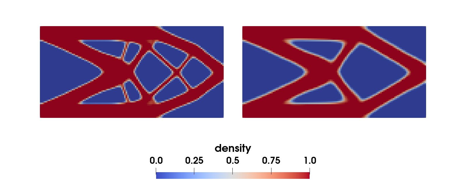
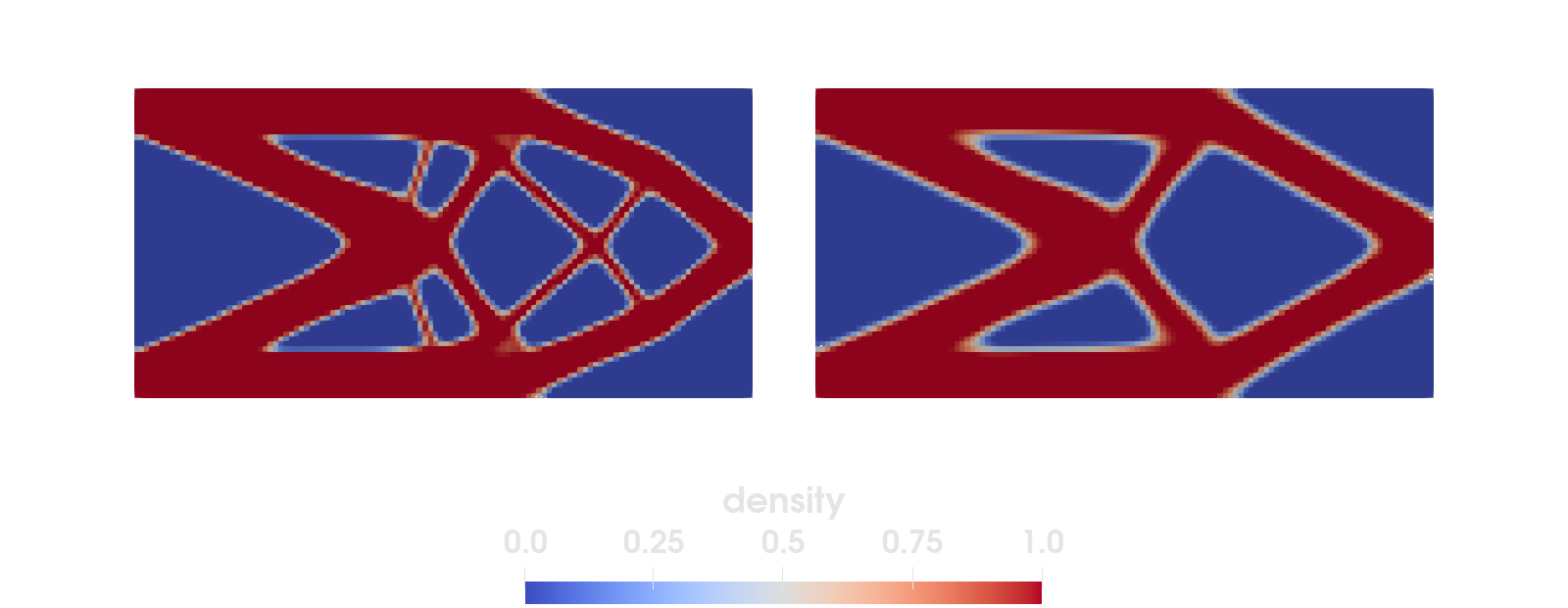
Figure 2: Optimization results of the bending beam for smaller (left) and larger (right) value of the regularization parameter $\beta$.

To prove mesh independence, the user could vary the mesh resolution and compare the results.

References

Plain program

Here follows a version of the program without any comments. The file is also available here: topology_optimization.jl.

using Ferrite, SparseArrays, LinearAlgebra, Tensors, Printf, VTKHDFfunction create_grid(n)    corners = [        Vec{2}((0.0, 0.0)),        Vec{2}((2.0, 0.0)),        Vec{2}((2.0, 1.0)),        Vec{2}((0.0, 1.0)),    ]    grid = generate_grid(Quadrilateral, (2 * n, n), corners)    # node- and facetsets for boundary conditions    addnodeset!(grid, "clamped", x -> x[1] ≈ 0.0)    addfacetset!(grid, "traction", x -> x[1] ≈ 2.0 && norm(x[2] - 0.5) <= 0.05)    return gridendfunction create_values()    # quadrature rules    qr = QuadratureRule{RefQuadrilateral}(2)    facet_qr = FacetQuadratureRule{RefQuadrilateral}(2)    # cell and facetvalues for u    ip = Lagrange{RefQuadrilateral, 1}()^2    cellvalues = CellValues(qr, ip)    facetvalues = FacetValues(facet_qr, ip)    return cellvalues, facetvaluesendfunction create_dofhandler(grid)    dh = DofHandler(grid)    add!(dh, :u, Lagrange{RefQuadrilateral, 1}()^2) # displacement    close!(dh)    return dhendfunction create_bc(dh, grid)    dbc = ConstraintHandler(dh)    add!(dbc, Dirichlet(:u, getnodeset(grid, "clamped"), (x, t) -> zero(Vec{2}), [1, 2]))    close!(dbc)    t = 0.0    update!(dbc, t)    return dbcendstruct MaterialParameters{T, S <: SymmetricTensor{4, 2, T}}    C::S    χ_min::T    p::T    β::T    η::Tendfunction MaterialParameters(E, ν, χ_min, p, β, η)    δ(i, j) = i == j ? 1.0 : 0.0 # helper function    G = E / 2(1 + ν) # =μ    λ = E * ν / (1 - ν^2) # correction for plane stress included    C = SymmetricTensor{4, 2}((i, j, k, l) -> λ * δ(i, j) * δ(k, l) + G * (δ(i, k) * δ(j, l) + δ(i, l) * δ(j, k)))    return MaterialParameters(C, χ_min, p, β, η)endmutable struct MaterialState{T, S <: AbstractArray{SymmetricTensor{2, 2, T, 3}, 1}}    χ::T # density    ε::S # strain in each quadrature pointendfunction MaterialState(ρ, n_qp)    return MaterialState(ρ, Array{SymmetricTensor{2, 2, Float64, 3}, 1}(undef, n_qp))endfunction update_material_states!(χn1, states, dh)    for (element, state) in zip(CellIterator(dh), states)        state.χ = χn1[cellid(element)]    end    returnendfunction compute_driving_forces(states, mp, dh, χn)    pΨ = zeros(length(states))    for (element, state) in zip(CellIterator(dh), states)        i = cellid(element)        ε = sum(state.ε) / length(state.ε) # average element strain        pΨ[i] = 1 / 2 * mp.p * χn[i]^(mp.p - 1) * (ε ⊡ mp.C ⊡ ε)    end    return pΨendfunction compute_densities(states, dh)    χn = zeros(length(states))    for (element, state) in zip(CellIterator(dh), states)        i = cellid(element)        χn[i] = state.χ    end    return χnendfunction cache_neighborhood(grid, topology)    opp = (3, 4, 1, 2) # opposite facet of facets 1, 2, 3, 4    neighborhood = Ferrite.get_facet_facet_neighborhood(topology, grid)    nbgs = Vector{Vector{Int}}(undef, getncells(grid))    for element in CellIterator(grid)        i = cellid(element)        _nfacets = nfacets(element)        nbg = zeros(Int, _nfacets)        for j in 1:_nfacets            neighbor_facets = neighborhood[i, j]            if !isempty(neighbor_facets)                nbg[j] = neighbor_facets[1][1] # assuming only one facet neighbor per cell            else # boundary facet                nbg[j] = neighborhood[i, opp[j]][1][1]            end        end        nbgs[i] = nbg    end    return nbgsendfunction approximate_laplacian(nbgs, χn, Δh)    ∇²χ = zeros(length(nbgs))    for i in 1:length(nbgs)        nbg = nbgs[i]        ∇²χ[i] = (χn[nbg[1]] + χn[nbg[2]] + χn[nbg[3]] + χn[nbg[4]] - 4 * χn[i]) / (Δh^2)    end    return ∇²χendfunction compute_χn1(χn, Δχ, ρ, ηs, χ_min)    n_el = length(χn)    χ_trial = zeros(n_el)    ρ_trial = 0.0    λ_lower = minimum(Δχ) - ηs    λ_upper = maximum(Δχ) + ηs    λ_trial = 0.0    while abs(ρ - ρ_trial) > 1.0e-7        for i in 1:n_el            Δχt = 1 / ηs * (Δχ[i] - λ_trial)            χ_trial[i] = max(χ_min, min(1.0, χn[i] + Δχt))        end        ρ_trial = 0.0        for i in 1:n_el            ρ_trial += χ_trial[i] / n_el        end        if ρ_trial > ρ            λ_lower = λ_trial        elseif ρ_trial < ρ            λ_upper = λ_trial        end        λ_trial = 1 / 2 * (λ_upper + λ_lower)    end    return χ_trialendfunction compute_average_driving_force(mp, pΨ, χn)    n = length(pΨ)    w = zeros(n)    for i in 1:n        w[i] = (χn[i] - mp.χ_min) * (1 - χn[i])    end    p_Ω = sum(w .* pΨ) / sum(w) # average driving force    return p_Ωendfunction update_density(dh, states, mp, ρ, neighborhoods, Δh)    n_j = Int(ceil(6 * mp.β / (mp.η * Δh^2))) # iterations needed for stability    χn = compute_densities(states, dh) # old density field    χn1 = zeros(length(χn))    for j in 1:n_j        ∇²χ = approximate_laplacian(neighborhoods, χn, Δh) # Laplacian        pΨ = compute_driving_forces(states, mp, dh, χn) # driving forces        p_Ω = compute_average_driving_force(mp, pΨ, χn) # average driving force        Δχ = pΨ / p_Ω + mp.β * ∇²χ        χn1 = compute_χn1(χn, Δχ, ρ, mp.η, mp.χ_min)        if j < n_j            χn[:] = χn1[:]        end    end    return χn1endfunction doassemble!(cellvalues::CellValues, facetvalues::FacetValues, K::SparseMatrixCSC, grid::Grid, dh::DofHandler, mp::MaterialParameters, u, states)    r = zeros(ndofs(dh))    assembler = start_assemble(K, r)    nu = getnbasefunctions(cellvalues)    re = zeros(nu) # local residual vector    Ke = zeros(nu, nu) # local stiffness matrix    for (element, state) in zip(CellIterator(dh), states)        fill!(Ke, 0)        fill!(re, 0)        eldofs = celldofs(element)        ue = u[eldofs]        elmt!(Ke, re, element, cellvalues, facetvalues, grid, mp, ue, state)        assemble!(assembler, celldofs(element), Ke, re)    end    return K, rendfunction elmt!(Ke, re, element, cellvalues, facetvalues, grid, mp, ue, state)    n_basefuncs = getnbasefunctions(cellvalues)    reinit!(cellvalues, element)    χ = state.χ    # We only assemble lower half triangle of the stiffness matrix and then symmetrize it.    @inbounds for q_point in 1:getnquadpoints(cellvalues)        dΩ = getdetJdV(cellvalues, q_point)        state.ε[q_point] = function_symmetric_gradient(cellvalues, q_point, ue)        for i in 1:n_basefuncs            δεi = shape_symmetric_gradient(cellvalues, q_point, i)            for j in 1:i                δεj = shape_symmetric_gradient(cellvalues, q_point, j)                Ke[i, j] += (χ)^(mp.p) * (δεi ⊡ mp.C ⊡ δεj) * dΩ            end            re[i] += (-δεi ⊡ ((χ)^(mp.p) * mp.C ⊡ state.ε[q_point])) * dΩ        end    end    symmetrize_lower!(Ke)    @inbounds for facet in 1:nfacets(getcells(grid, cellid(element)))        if (cellid(element), facet) ∈ getfacetset(grid, "traction")            reinit!(facetvalues, element, facet)            t = Vec((0.0, -1.0)) # force pointing downwards            for q_point in 1:getnquadpoints(facetvalues)                dΓ = getdetJdV(facetvalues, q_point)                for i in 1:n_basefuncs                    δu = shape_value(facetvalues, q_point, i)                    re[i] += (δu ⋅ t) * dΓ                end            end        end    end    returnendfunction symmetrize_lower!(K)    for i in 1:size(K, 1)        for j in (i + 1):size(K, 1)            K[i, j] = K[j, i]        end    end    returnendfunction topopt(ra, ρ, n, filename; output = false)    # material    mp = MaterialParameters(210.0e3, 0.3, 1.0e-3, 3.0, ra^2, 15.0)    # grid, dofhandler, boundary condition    grid = create_grid(n)    dh = create_dofhandler(grid)    Δh = 1 / n # element edge length    dbc = create_bc(dh, grid)    # cellvalues    cellvalues, facetvalues = create_values()    # Pre-allocate solution vectors, etc.    n_dofs = ndofs(dh) # total number of dofs    u = zeros(n_dofs) # solution vector    un = zeros(n_dofs) # previous solution vector    Δu = zeros(n_dofs)  # previous displacement correction    ΔΔu = zeros(n_dofs) # new displacement correction    # create material states    states = [MaterialState(ρ, getnquadpoints(cellvalues)) for _ in 1:getncells(grid)]    χ = zeros(getncells(grid))    r = zeros(n_dofs) # residual    K = allocate_matrix(dh) # stiffness matrix    i_max = 300 ## maximum number of iteration steps    tol = 1.0e-4    compliance = 0.0    compliance_0 = 0.0    compliance_n = 0.0    conv = false    topology = ExclusiveTopology(grid)    neighborhoods = cache_neighborhood(grid, topology)    # Newton-Raphson loop    NEWTON_TOL = 1.0e-8    print("\n Starting Newton iterations\n")    # When `output = true` the density of every iteration is stored as one time    # step in a single temporal VTKHDF file so the evolution can be animated.    vtkhdf = output ? VTKHDFGridFile(string(filename, ".vtkhdf"), grid; temporal = true) : nothing    for it in 1:i_max        apply_zero!(u, dbc)        newton_itr = -1        while true            newton_itr += 1            if newton_itr > 10                error("Reached maximum Newton iterations, aborting")                break            end            # current guess            u .= un .+ Δu            K, r = doassemble!(cellvalues, facetvalues, K, grid, dh, mp, u, states)            norm_r = norm(r[Ferrite.free_dofs(dbc)])            if (norm_r) < NEWTON_TOL                break            end            apply_zero!(K, r, dbc)            ΔΔu = Symmetric(K) \ r            apply_zero!(ΔΔu, dbc)            Δu .+= ΔΔu        end # of loop while NR-Iteration        # calculate compliance        compliance = 1 / 2 * u' * K * u        if it == 1            compliance_0 = compliance        end        # check convergence criterion (twice!)        if abs(compliance - compliance_n) / compliance < tol            if conv                println("Converged at iteration number: ", it)                break            else                conv = true            end        else            conv = false        end        # update density        χ = update_density(dh, states, mp, ρ, neighborhoods, Δh)        # update old displacement, density and compliance        un .= u        Δu .= 0.0        update_material_states!(χ, states, dh)        compliance_n = compliance        # output during calculation        if output            write_timestep(vtkhdf, Float64(it)) do vtk                write_cell_data(vtk, χ, "density")            end        end    end    output && close(vtkhdf)    # export converged results    if !output        VTKGridFile(filename, grid) do vtk            write_cell_data(vtk, χ, "density")        end    end    @printf "Rel. stiffness: %.4f \n" compliance^(-1) / compliance_0^(-1)    returnend@time topopt(0.03, 0.5, 60, "large_radius"; output = false);#topopt(0.02, 0.5, 60, "topopt_animation"; output=true); # can be used to create animationstopopt(0.03, 0.5, 60, "topopt_frames"; output = true); #src iteration series for the docs animation (docs/screenshots.py)

This page was generated using Literate.jl.