Von Mises plasticity

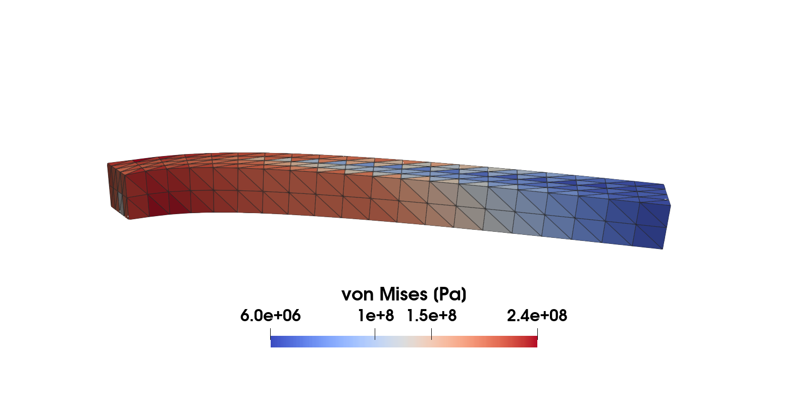
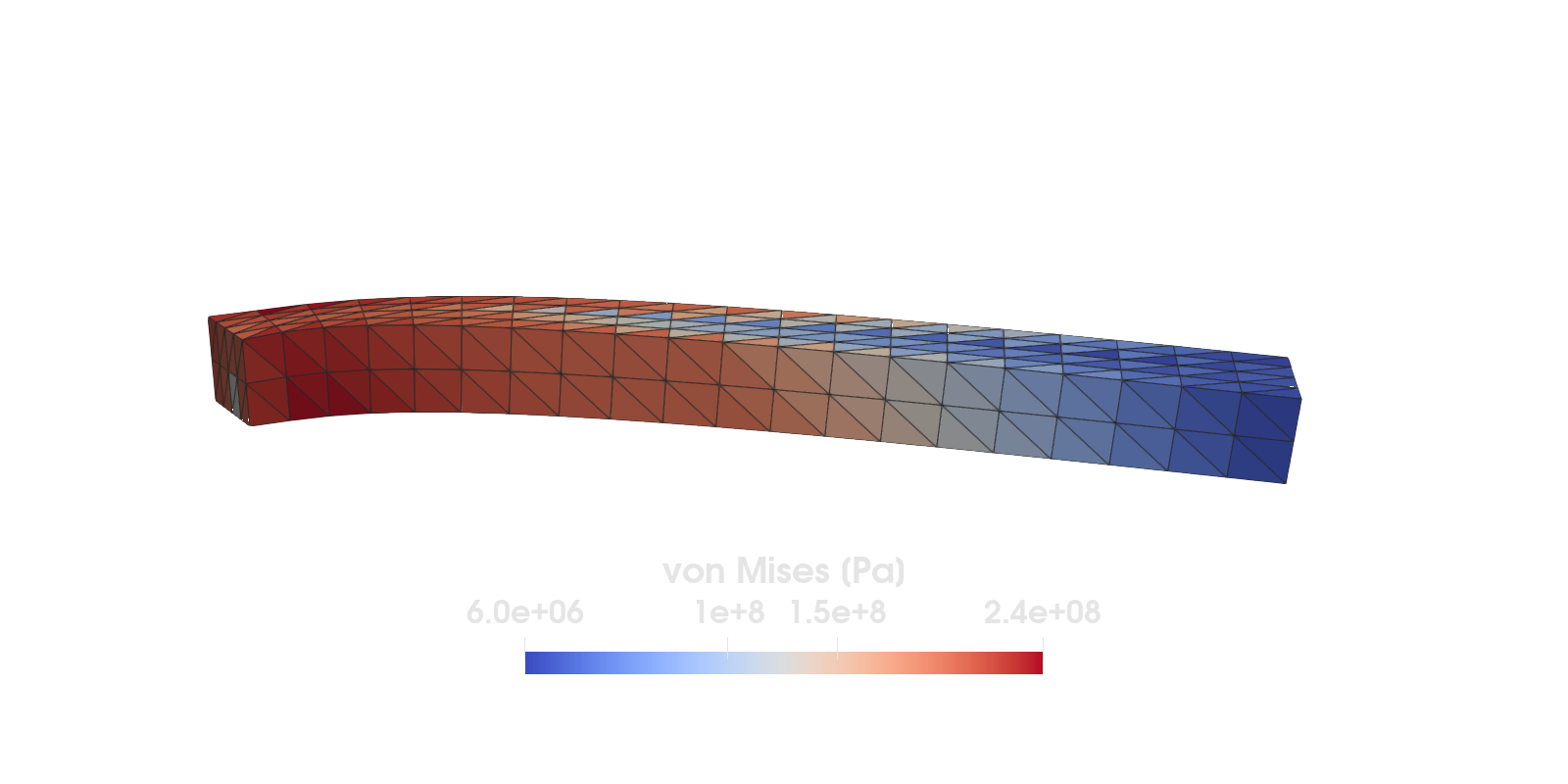
Shows the von Mises stress distribution in a cantilever beam.

Figure 1. A coarse mesh solution of a cantilever beam subjected to a load causing plastic deformations. The initial yield limit is 200 MPa but due to hardening it increases up to approximately 240 MPa.

Tip

This example is also available as a Jupyter notebook: plasticity.ipynb.

Introduction

This example illustrates the use of a nonlinear material model in Ferrite. The particular model is von Mises plasticity (also know as J₂-plasticity) with isotropic hardening. The model is fully 3D, meaning that no assumptions like plane stress or plane strain are introduced.

Also note that the theory of the model is not described here, instead one is referred to standard textbooks on material modeling.

To illustrate the use of the plasticity model, we setup and solve a FE-problem consisting of a cantilever beam loaded at its free end. But first, we shortly describe the parts of the implementation dealing with the material modeling.

Material modeling

This section describes the structs and methods used to implement the material model

Material parameters and state variables

Start by loading some necessary packages

using Ferrite, Tensors, SparseArrays, LinearAlgebra, Printf

We define a J₂-plasticity-material, containing material parameters and the elastic stiffness Dᵉ (since it is constant)

struct J2Plasticity{T, S <: SymmetricTensor{4, 3, T}}
    G::T  # Shear modulus
    K::T  # Bulk modulus
    σ₀::T # Initial yield limit
    H::T  # Hardening modulus
    Dᵉ::S # Elastic stiffness tensor
end;

Next, we define a constructor for the material instance.

function J2Plasticity(E, ν, σ₀, H)
    δ(i, j) = i == j ? 1.0 : 0.0 # helper function
    G = E / 2(1 + ν)
    K = E / 3(1 - 2ν)

    Isymdev(i, j, k, l) = 0.5 * (δ(i, k) * δ(j, l) + δ(i, l) * δ(j, k)) - 1.0 / 3.0 * δ(i, j) * δ(k, l)
    temp(i, j, k, l) = 2.0G * (0.5 * (δ(i, k) * δ(j, l) + δ(i, l) * δ(j, k)) + ν / (1.0 - 2.0ν) * δ(i, j) * δ(k, l))
    Dᵉ = SymmetricTensor{4, 3}(temp)
    return J2Plasticity(G, K, σ₀, H, Dᵉ)
end;

Note

Above, we defined a constructor J2Plasticity(E, ν, σ₀, H) in terms of the more common material parameters $E$ and $ν$ - simply as a convenience for the user.

Define a struct to store the material state for a Gauss point.

struct MaterialState{T, S <: SecondOrderTensor{3, T}}
    # Store "converged" values
    ϵᵖ::S # plastic strain
    σ::S # stress
    k::T # hardening variable
end

Constructor for initializing a material state. Every quantity is set to zero.

function MaterialState()
    return MaterialState(
        zero(SymmetricTensor{2, 3}),
        zero(SymmetricTensor{2, 3}),
        0.0
    )
end

Main.MaterialState

For later use, during the post-processing step, we define a function to compute the von Mises effective stress.

function vonMises(σ)
    s = dev(σ)
    return sqrt(3.0 / 2.0 * s ⊡ s)
end;

Constitutive driver

This is the actual method which computes the stress and material tangent stiffness in a given integration point. Input is the current strain and the material state from the previous timestep.

function compute_stress_tangent(ϵ::SymmetricTensor{2, 3}, material::J2Plasticity, state::MaterialState)
    # unpack some material parameters
    G = material.G
    H = material.H

    # We use (•)ᵗ to denote *trial*-values
    σᵗ = material.Dᵉ ⊡ (ϵ - state.ϵᵖ) # trial-stress
    sᵗ = dev(σᵗ)         # deviatoric part of trial-stress
    J₂ = 0.5 * sᵗ ⊡ sᵗ   # second invariant of sᵗ
    σᵗₑ = sqrt(3.0 * J₂) # effective trial-stress (von Mises stress)
    σʸ = material.σ₀ + H * state.k # Previous yield limit

    φᵗ = σᵗₑ - σʸ # Trial-value of the yield surface

    if φᵗ < 0.0 # elastic loading
        return σᵗ, material.Dᵉ, MaterialState(state.ϵᵖ, σᵗ, state.k)
    else # plastic loading
        h = H + 3G
        μ = φᵗ / h # plastic multiplier

        c1 = 1 - 3G * μ / σᵗₑ
        s = c1 * sᵗ           # updated deviatoric stress
        σ = s + vol(σᵗ)       # updated stress

        # Compute algorithmic tangent stiffness ``D = \frac{\Delta \sigma }{\Delta \epsilon}``
        κ = H * (state.k + μ) # drag stress
        σₑ = material.σ₀ + κ  # updated yield surface

        δ(i, j) = i == j ? 1.0 : 0.0
        Isymdev(i, j, k, l) = 0.5 * (δ(i, k) * δ(j, l) + δ(i, l) * δ(j, k)) - 1.0 / 3.0 * δ(i, j) * δ(k, l)
        Q(i, j, k, l) = Isymdev(i, j, k, l) - 3.0 / (2.0 * σₑ^2) * s[i, j] * s[k, l]
        b = (3G * μ / σₑ) / (1.0 + 3G * μ / σₑ)

        Dtemp(i, j, k, l) = -2G * b * Q(i, j, k, l) - 9G^2 / (h * σₑ^2) * s[i, j] * s[k, l]
        D = material.Dᵉ + SymmetricTensor{4, 3}(Dtemp)

        # Return new state
        Δϵᵖ = 3 / 2 * μ / σₑ * s # plastic strain
        ϵᵖ = state.ϵᵖ + Δϵᵖ      # plastic strain
        k = state.k + μ          # hardening variable
        return σ, D, MaterialState(ϵᵖ, σ, k)
    end
end

compute_stress_tangent (generic function with 1 method)

FE-problem

What follows are methods for assembling and solving the FE-problem.

function create_values(interpolation)
    # setup quadrature rules
    qr = QuadratureRule{RefTetrahedron}(2)
    facet_qr = FacetQuadratureRule{RefTetrahedron}(3)

    # cell and facetvalues for u
    cellvalues_u = CellValues(qr, interpolation)
    facetvalues_u = FacetValues(facet_qr, interpolation)

    return cellvalues_u, facetvalues_u
end;

Add degrees of freedom

function create_dofhandler(grid, interpolation)
    dh = DofHandler(grid)
    add!(dh, :u, interpolation) # add a displacement field with 3 components
    close!(dh)
    return dh
end

create_dofhandler (generic function with 1 method)

Boundary conditions

function create_bc(dh, grid)
    dbcs = ConstraintHandler(dh)
    # Clamped on the left side
    dofs = [1, 2, 3]
    dbc = Dirichlet(:u, getfacetset(grid, "left"), (x, t) -> [0.0, 0.0, 0.0], dofs)
    add!(dbcs, dbc)
    close!(dbcs)
    return dbcs
end;

Assembling of element contributions

Residual vector r
Tangent stiffness K

function doassemble!(
        K::SparseMatrixCSC, r::Vector, cellvalues::CellValues, dh::DofHandler,
        material::J2Plasticity, u, states, states_old
    )
    assembler = start_assemble(K, r)
    nu = getnbasefunctions(cellvalues)
    re = zeros(nu)     # element residual vector
    ke = zeros(nu, nu) # element tangent matrix

    for (i, cell) in enumerate(CellIterator(dh))
        fill!(ke, 0)
        fill!(re, 0)
        eldofs = celldofs(cell)
        ue = u[eldofs]
        state = @view states[:, i]
        state_old = @view states_old[:, i]
        assemble_cell!(ke, re, cell, cellvalues, material, ue, state, state_old)
        assemble!(assembler, eldofs, ke, re)
    end
    return K, r
end

doassemble! (generic function with 1 method)

Compute element contribution to the residual and the tangent.

Note

Due to symmetry, we only compute the lower half of the tangent and then symmetrize it.

function assemble_cell!(Ke, re, cell, cellvalues, material, ue, state, state_old)
    n_basefuncs = getnbasefunctions(cellvalues)
    reinit!(cellvalues, cell)

    for q_point in 1:getnquadpoints(cellvalues)
        # For each integration point, compute stress and material stiffness
        ϵ = function_symmetric_gradient(cellvalues, q_point, ue) # Total strain
        σ, D, state[q_point] = compute_stress_tangent(ϵ, material, state_old[q_point])

        dΩ = getdetJdV(cellvalues, q_point)
        for i in 1:n_basefuncs
            δϵ = shape_symmetric_gradient(cellvalues, q_point, i)
            re[i] += (δϵ ⊡ σ) * dΩ # add internal force to residual
            for j in 1:i # loop only over lower half
                Δϵ = shape_symmetric_gradient(cellvalues, q_point, j)
                Ke[i, j] += δϵ ⊡ D ⊡ Δϵ * dΩ
            end
        end
    end
    symmetrize_lower!(Ke)
    return
end

assemble_cell! (generic function with 1 method)

Helper function to symmetrize the material tangent

function symmetrize_lower!(K)
    for i in 1:size(K, 1)
        for j in (i + 1):size(K, 1)
            K[i, j] = K[j, i]
        end
    end
    return
end;

function doassemble_neumann!(r, dh, facetset, facetvalues, t)
    n_basefuncs = getnbasefunctions(facetvalues)
    re = zeros(n_basefuncs)                      # element residual vector
    for fc in FacetIterator(dh, facetset)
        # Add traction as a negative contribution to the element residual `re`:
        reinit!(facetvalues, fc)
        fill!(re, 0)
        for q_point in 1:getnquadpoints(facetvalues)
            dΓ = getdetJdV(facetvalues, q_point)
            for i in 1:n_basefuncs
                δu = shape_value(facetvalues, q_point, i)
                re[i] -= (δu ⋅ t) * dΓ
            end
        end
        assemble!(r, celldofs(fc), re)
    end
    return r
end

doassemble_neumann! (generic function with 1 method)

Define a function which solves the FE-problem.

function solve()
    # Define material parameters
    E = 200.0e9  # [Pa]
    H = E / 20   # [Pa]
    ν = 0.3      # [-]
    σ₀ = 200.0e6 # [Pa]
    material = J2Plasticity(E, ν, σ₀, H)

    L = 10.0 # beam length [m]
    w = 1.0  # beam width [m]
    h = 1.0  # beam height[m]
    n_timesteps = 10
    u_max = zeros(n_timesteps)
    traction_magnitude = 1.0e7 * range(0.5, 1.0, length = n_timesteps)

    # Create geometry, dofs and boundary conditions
    n = 2
    nels = (10n, n, 2n) # number of elements in each spatial direction
    P1 = Vec((0.0, 0.0, 0.0))  # start point for geometry
    P2 = Vec((L, w, h))        # end point for geometry
    grid = generate_grid(Tetrahedron, nels, P1, P2)
    interpolation = Lagrange{RefTetrahedron, 1}()^3

    dh = create_dofhandler(grid, interpolation) # helper function defined above
    dbcs = create_bc(dh, grid) # create Dirichlet boundary-conditions

    cellvalues, facetvalues = create_values(interpolation)

    # Pre-allocate solution vectors, etc.
    n_dofs = ndofs(dh)  # total number of dofs
    u = zeros(n_dofs)   # solution vector
    Δu = zeros(n_dofs)  # displacement correction
    r = zeros(n_dofs)   # residual
    K = allocate_matrix(dh) # tangent stiffness matrix

    # Create material states. One array for each cell, where each element is an array of material-
    # states - one for each integration point
    nqp = getnquadpoints(cellvalues)
    states = [MaterialState() for _ in 1:nqp, _ in 1:getncells(grid)]
    states_old = [MaterialState() for _ in 1:nqp, _ in 1:getncells(grid)]

    # Newton-Raphson loop
    NEWTON_TOL = 1 # 1 N
    print("\n Starting Newton iterations:\n")

    for timestep in 1:n_timesteps
        t = timestep # actual time (used for evaluating d-bndc)
        traction = Vec((0.0, 0.0, traction_magnitude[timestep]))
        newton_itr = -1
        print("\n Time step @time = $timestep:\n")
        update!(dbcs, t) # evaluates the D-bndc at time t
        apply!(u, dbcs)  # set the prescribed values in the solution vector

        while true
            newton_itr += 1
            if newton_itr > 8
                error("Reached maximum Newton iterations, aborting")
                break
            end
            # Tangent and residual contribution from the cells (volume integral)
            doassemble!(K, r, cellvalues, dh, material, u, states, states_old)
            # Residual contribution from the Neumann boundary (surface integral)
            doassemble_neumann!(r, dh, getfacetset(grid, "right"), facetvalues, traction)
            norm_r = norm(r[Ferrite.free_dofs(dbcs)])

            print("Iteration: $newton_itr \tresidual: $(@sprintf("%.8f", norm_r))\n")
            if norm_r < NEWTON_TOL
                break
            end

            apply_zero!(K, r, dbcs)
            Δu = Symmetric(K) \ r
            u -= Δu
        end

        # Update the old states with the converged values for next timestep
        states_old .= states

        u_max[timestep] = maximum(abs, u) # maximum displacement in current timestep
    end

    # ## Postprocessing
    # Only a vtu-file corresponding to the last time-step is exported.
    #
    # The following is a quick (and dirty) way of extracting average cell data for export.
    mises_values = zeros(getncells(grid))
    κ_values = zeros(getncells(grid))
    for (el, cell_states) in enumerate(eachcol(states))
        for state in cell_states
            mises_values[el] += vonMises(state.σ)
            κ_values[el] += state.k * material.H
        end
        mises_values[el] /= length(cell_states) # average von Mises stress
        κ_values[el] /= length(cell_states)     # average drag stress
    end
    VTKGridFile("plasticity", dh) do vtk
        write_solution(vtk, dh, u) # displacement field
        write_cell_data(vtk, mises_values, "von Mises [Pa]")
        write_cell_data(vtk, κ_values, "Drag stress [Pa]")
    end

    return u_max, traction_magnitude
end

solve (generic function with 1 method)

Solve the FE-problem and for each time-step extract maximum displacement and the corresponding traction load. Also compute the limit-traction-load

u_max, traction_magnitude = solve();


 Starting Newton iterations:

 Time step @time = 1:
Iteration: 0 	residual: 1435838.41167605
Iteration: 1 	residual: 118655.22433757
Iteration: 2 	residual: 59.50456051
Iteration: 3 	residual: 0.00002618

 Time step @time = 2:
Iteration: 0 	residual: 159537.60129714
Iteration: 1 	residual: 1694313.86971151
Iteration: 2 	residual: 61777.44063586
Iteration: 3 	residual: 14.34471355
Iteration: 4 	residual: 0.00001201

 Time step @time = 3:
Iteration: 0 	residual: 159537.60129709
Iteration: 1 	residual: 2870967.96937456
Iteration: 2 	residual: 83501.38262846
Iteration: 3 	residual: 36.06150658
Iteration: 4 	residual: 0.00001919

 Time step @time = 4:
Iteration: 0 	residual: 159537.60129780
Iteration: 1 	residual: 4477547.43401468
Iteration: 2 	residual: 148240.13900304
Iteration: 3 	residual: 128.89783066
Iteration: 4 	residual: 0.00016901

 Time step @time = 5:
Iteration: 0 	residual: 159537.60129738
Iteration: 1 	residual: 4588016.54576168
Iteration: 2 	residual: 617974.22614660
Iteration: 3 	residual: 1547.60759281
Iteration: 4 	residual: 0.01582895

 Time step @time = 6:
Iteration: 0 	residual: 159537.60129708
Iteration: 1 	residual: 6104778.59010419
Iteration: 2 	residual: 1789878.33703872
Iteration: 3 	residual: 18862.06803338
Iteration: 4 	residual: 2.19496915
Iteration: 5 	residual: 0.00001943

 Time step @time = 7:
Iteration: 0 	residual: 159537.60129756
Iteration: 1 	residual: 7017230.56449254
Iteration: 2 	residual: 1780082.38831216
Iteration: 3 	residual: 15343.77854601
Iteration: 4 	residual: 1.43921960
Iteration: 5 	residual: 0.00002599

 Time step @time = 8:
Iteration: 0 	residual: 159537.60129763
Iteration: 1 	residual: 8179652.08583717
Iteration: 2 	residual: 2162977.64320989
Iteration: 3 	residual: 19555.20410310
Iteration: 4 	residual: 2.68797184
Iteration: 5 	residual: 0.00002899

 Time step @time = 9:
Iteration: 0 	residual: 159537.60129685
Iteration: 1 	residual: 8622256.63871769
Iteration: 2 	residual: 2009697.23769223
Iteration: 3 	residual: 14905.08785988
Iteration: 4 	residual: 1.57894129
Iteration: 5 	residual: 0.00003398

 Time step @time = 10:
Iteration: 0 	residual: 159537.60129656
Iteration: 1 	residual: 9505824.59004884
Iteration: 2 	residual: 1712399.15379926
Iteration: 3 	residual: 33813.52525863
Iteration: 4 	residual: 4.35721836
Iteration: 5 	residual: 0.00004462

Finally we plot the load-displacement curve.

using Plots
plot(
    vcat(0.0, u_max),                # add the origin as a point
    vcat(0.0, traction_magnitude),
    linewidth = 2,
    title = "Traction-displacement",
    label = nothing,
    markershape = :auto
)
ylabel!("Traction [Pa]")
xlabel!("Maximum deflection [m]")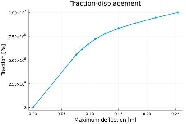

Figure 2. Load-displacement-curve for the beam, showing a clear decrease in stiffness as more material starts to yield.

Plain program

Here follows a version of the program without any comments. The file is also available here: plasticity.jl.

using Ferrite, Tensors, SparseArrays, LinearAlgebra, Printf

struct J2Plasticity{T, S <: SymmetricTensor{4, 3, T}}
    G::T  # Shear modulus
    K::T  # Bulk modulus
    σ₀::T # Initial yield limit
    H::T  # Hardening modulus
    Dᵉ::S # Elastic stiffness tensor
end;

function J2Plasticity(E, ν, σ₀, H)
    δ(i, j) = i == j ? 1.0 : 0.0 # helper function
    G = E / 2(1 + ν)
    K = E / 3(1 - 2ν)

    Isymdev(i, j, k, l) = 0.5 * (δ(i, k) * δ(j, l) + δ(i, l) * δ(j, k)) - 1.0 / 3.0 * δ(i, j) * δ(k, l)
    temp(i, j, k, l) = 2.0G * (0.5 * (δ(i, k) * δ(j, l) + δ(i, l) * δ(j, k)) + ν / (1.0 - 2.0ν) * δ(i, j) * δ(k, l))
    Dᵉ = SymmetricTensor{4, 3}(temp)
    return J2Plasticity(G, K, σ₀, H, Dᵉ)
end;

struct MaterialState{T, S <: SecondOrderTensor{3, T}}
    # Store "converged" values
    ϵᵖ::S # plastic strain
    σ::S # stress
    k::T # hardening variable
end

function MaterialState()
    return MaterialState(
        zero(SymmetricTensor{2, 3}),
        zero(SymmetricTensor{2, 3}),
        0.0
    )
end

function vonMises(σ)
    s = dev(σ)
    return sqrt(3.0 / 2.0 * s ⊡ s)
end;

function compute_stress_tangent(ϵ::SymmetricTensor{2, 3}, material::J2Plasticity, state::MaterialState)
    # unpack some material parameters
    G = material.G
    H = material.H

    # We use (•)ᵗ to denote *trial*-values
    σᵗ = material.Dᵉ ⊡ (ϵ - state.ϵᵖ) # trial-stress
    sᵗ = dev(σᵗ)         # deviatoric part of trial-stress
    J₂ = 0.5 * sᵗ ⊡ sᵗ   # second invariant of sᵗ
    σᵗₑ = sqrt(3.0 * J₂) # effective trial-stress (von Mises stress)
    σʸ = material.σ₀ + H * state.k # Previous yield limit

    φᵗ = σᵗₑ - σʸ # Trial-value of the yield surface

    if φᵗ < 0.0 # elastic loading
        return σᵗ, material.Dᵉ, MaterialState(state.ϵᵖ, σᵗ, state.k)
    else # plastic loading
        h = H + 3G
        μ = φᵗ / h # plastic multiplier

        c1 = 1 - 3G * μ / σᵗₑ
        s = c1 * sᵗ           # updated deviatoric stress
        σ = s + vol(σᵗ)       # updated stress

        # Compute algorithmic tangent stiffness ``D = \frac{\Delta \sigma }{\Delta \epsilon}``
        κ = H * (state.k + μ) # drag stress
        σₑ = material.σ₀ + κ  # updated yield surface

        δ(i, j) = i == j ? 1.0 : 0.0
        Isymdev(i, j, k, l) = 0.5 * (δ(i, k) * δ(j, l) + δ(i, l) * δ(j, k)) - 1.0 / 3.0 * δ(i, j) * δ(k, l)
        Q(i, j, k, l) = Isymdev(i, j, k, l) - 3.0 / (2.0 * σₑ^2) * s[i, j] * s[k, l]
        b = (3G * μ / σₑ) / (1.0 + 3G * μ / σₑ)

        Dtemp(i, j, k, l) = -2G * b * Q(i, j, k, l) - 9G^2 / (h * σₑ^2) * s[i, j] * s[k, l]
        D = material.Dᵉ + SymmetricTensor{4, 3}(Dtemp)

        # Return new state
        Δϵᵖ = 3 / 2 * μ / σₑ * s # plastic strain
        ϵᵖ = state.ϵᵖ + Δϵᵖ      # plastic strain
        k = state.k + μ          # hardening variable
        return σ, D, MaterialState(ϵᵖ, σ, k)
    end
end

function create_values(interpolation)
    # setup quadrature rules
    qr = QuadratureRule{RefTetrahedron}(2)
    facet_qr = FacetQuadratureRule{RefTetrahedron}(3)

    # cell and facetvalues for u
    cellvalues_u = CellValues(qr, interpolation)
    facetvalues_u = FacetValues(facet_qr, interpolation)

    return cellvalues_u, facetvalues_u
end;

function create_dofhandler(grid, interpolation)
    dh = DofHandler(grid)
    add!(dh, :u, interpolation) # add a displacement field with 3 components
    close!(dh)
    return dh
end

function create_bc(dh, grid)
    dbcs = ConstraintHandler(dh)
    # Clamped on the left side
    dofs = [1, 2, 3]
    dbc = Dirichlet(:u, getfacetset(grid, "left"), (x, t) -> [0.0, 0.0, 0.0], dofs)
    add!(dbcs, dbc)
    close!(dbcs)
    return dbcs
end;

function doassemble!(
        K::SparseMatrixCSC, r::Vector, cellvalues::CellValues, dh::DofHandler,
        material::J2Plasticity, u, states, states_old
    )
    assembler = start_assemble(K, r)
    nu = getnbasefunctions(cellvalues)
    re = zeros(nu)     # element residual vector
    ke = zeros(nu, nu) # element tangent matrix

    for (i, cell) in enumerate(CellIterator(dh))
        fill!(ke, 0)
        fill!(re, 0)
        eldofs = celldofs(cell)
        ue = u[eldofs]
        state = @view states[:, i]
        state_old = @view states_old[:, i]
        assemble_cell!(ke, re, cell, cellvalues, material, ue, state, state_old)
        assemble!(assembler, eldofs, ke, re)
    end
    return K, r
end

function assemble_cell!(Ke, re, cell, cellvalues, material, ue, state, state_old)
    n_basefuncs = getnbasefunctions(cellvalues)
    reinit!(cellvalues, cell)

    for q_point in 1:getnquadpoints(cellvalues)
        # For each integration point, compute stress and material stiffness
        ϵ = function_symmetric_gradient(cellvalues, q_point, ue) # Total strain
        σ, D, state[q_point] = compute_stress_tangent(ϵ, material, state_old[q_point])

        dΩ = getdetJdV(cellvalues, q_point)
        for i in 1:n_basefuncs
            δϵ = shape_symmetric_gradient(cellvalues, q_point, i)
            re[i] += (δϵ ⊡ σ) * dΩ # add internal force to residual
            for j in 1:i # loop only over lower half
                Δϵ = shape_symmetric_gradient(cellvalues, q_point, j)
                Ke[i, j] += δϵ ⊡ D ⊡ Δϵ * dΩ
            end
        end
    end
    symmetrize_lower!(Ke)
    return
end

function symmetrize_lower!(K)
    for i in 1:size(K, 1)
        for j in (i + 1):size(K, 1)
            K[i, j] = K[j, i]
        end
    end
    return
end;

function doassemble_neumann!(r, dh, facetset, facetvalues, t)
    n_basefuncs = getnbasefunctions(facetvalues)
    re = zeros(n_basefuncs)                      # element residual vector
    for fc in FacetIterator(dh, facetset)
        # Add traction as a negative contribution to the element residual `re`:
        reinit!(facetvalues, fc)
        fill!(re, 0)
        for q_point in 1:getnquadpoints(facetvalues)
            dΓ = getdetJdV(facetvalues, q_point)
            for i in 1:n_basefuncs
                δu = shape_value(facetvalues, q_point, i)
                re[i] -= (δu ⋅ t) * dΓ
            end
        end
        assemble!(r, celldofs(fc), re)
    end
    return r
end

function solve()
    # Define material parameters
    E = 200.0e9  # [Pa]
    H = E / 20   # [Pa]
    ν = 0.3      # [-]
    σ₀ = 200.0e6 # [Pa]
    material = J2Plasticity(E, ν, σ₀, H)

    L = 10.0 # beam length [m]
    w = 1.0  # beam width [m]
    h = 1.0  # beam height[m]
    n_timesteps = 10
    u_max = zeros(n_timesteps)
    traction_magnitude = 1.0e7 * range(0.5, 1.0, length = n_timesteps)

    # Create geometry, dofs and boundary conditions
    n = 2
    nels = (10n, n, 2n) # number of elements in each spatial direction
    P1 = Vec((0.0, 0.0, 0.0))  # start point for geometry
    P2 = Vec((L, w, h))        # end point for geometry
    grid = generate_grid(Tetrahedron, nels, P1, P2)
    interpolation = Lagrange{RefTetrahedron, 1}()^3

    dh = create_dofhandler(grid, interpolation) # helper function defined above
    dbcs = create_bc(dh, grid) # create Dirichlet boundary-conditions

    cellvalues, facetvalues = create_values(interpolation)

    # Pre-allocate solution vectors, etc.
    n_dofs = ndofs(dh)  # total number of dofs
    u = zeros(n_dofs)   # solution vector
    Δu = zeros(n_dofs)  # displacement correction
    r = zeros(n_dofs)   # residual
    K = allocate_matrix(dh) # tangent stiffness matrix

    # Create material states. One array for each cell, where each element is an array of material-
    # states - one for each integration point
    nqp = getnquadpoints(cellvalues)
    states = [MaterialState() for _ in 1:nqp, _ in 1:getncells(grid)]
    states_old = [MaterialState() for _ in 1:nqp, _ in 1:getncells(grid)]

    # Newton-Raphson loop
    NEWTON_TOL = 1 # 1 N
    print("\n Starting Newton iterations:\n")

    for timestep in 1:n_timesteps
        t = timestep # actual time (used for evaluating d-bndc)
        traction = Vec((0.0, 0.0, traction_magnitude[timestep]))
        newton_itr = -1
        print("\n Time step @time = $timestep:\n")
        update!(dbcs, t) # evaluates the D-bndc at time t
        apply!(u, dbcs)  # set the prescribed values in the solution vector

        while true
            newton_itr += 1
            if newton_itr > 8
                error("Reached maximum Newton iterations, aborting")
                break
            end
            # Tangent and residual contribution from the cells (volume integral)
            doassemble!(K, r, cellvalues, dh, material, u, states, states_old)
            # Residual contribution from the Neumann boundary (surface integral)
            doassemble_neumann!(r, dh, getfacetset(grid, "right"), facetvalues, traction)
            norm_r = norm(r[Ferrite.free_dofs(dbcs)])

            print("Iteration: $newton_itr \tresidual: $(@sprintf("%.8f", norm_r))\n")
            if norm_r < NEWTON_TOL
                break
            end

            apply_zero!(K, r, dbcs)
            Δu = Symmetric(K) \ r
            u -= Δu
        end

        # Update the old states with the converged values for next timestep
        states_old .= states

        u_max[timestep] = maximum(abs, u) # maximum displacement in current timestep
    end

    # ## Postprocessing
    # Only a vtu-file corresponding to the last time-step is exported.
    #
    # The following is a quick (and dirty) way of extracting average cell data for export.
    mises_values = zeros(getncells(grid))
    κ_values = zeros(getncells(grid))
    for (el, cell_states) in enumerate(eachcol(states))
        for state in cell_states
            mises_values[el] += vonMises(state.σ)
            κ_values[el] += state.k * material.H
        end
        mises_values[el] /= length(cell_states) # average von Mises stress
        κ_values[el] /= length(cell_states)     # average drag stress
    end
    VTKGridFile("plasticity", dh) do vtk
        write_solution(vtk, dh, u) # displacement field
        write_cell_data(vtk, mises_values, "von Mises [Pa]")
        write_cell_data(vtk, κ_values, "Drag stress [Pa]")
    end

    return u_max, traction_magnitude
end

u_max, traction_magnitude = solve();

using Plots
plot(
    vcat(0.0, u_max),                # add the origin as a point
    vcat(0.0, traction_magnitude),
    linewidth = 2,
    title = "Traction-displacement",
    label = nothing,
    markershape = :auto
)
ylabel!("Traction [Pa]")
xlabel!("Maximum deflection [m]")

This page was generated using Literate.jl.