UnstructuredGrid: partitioned mesh

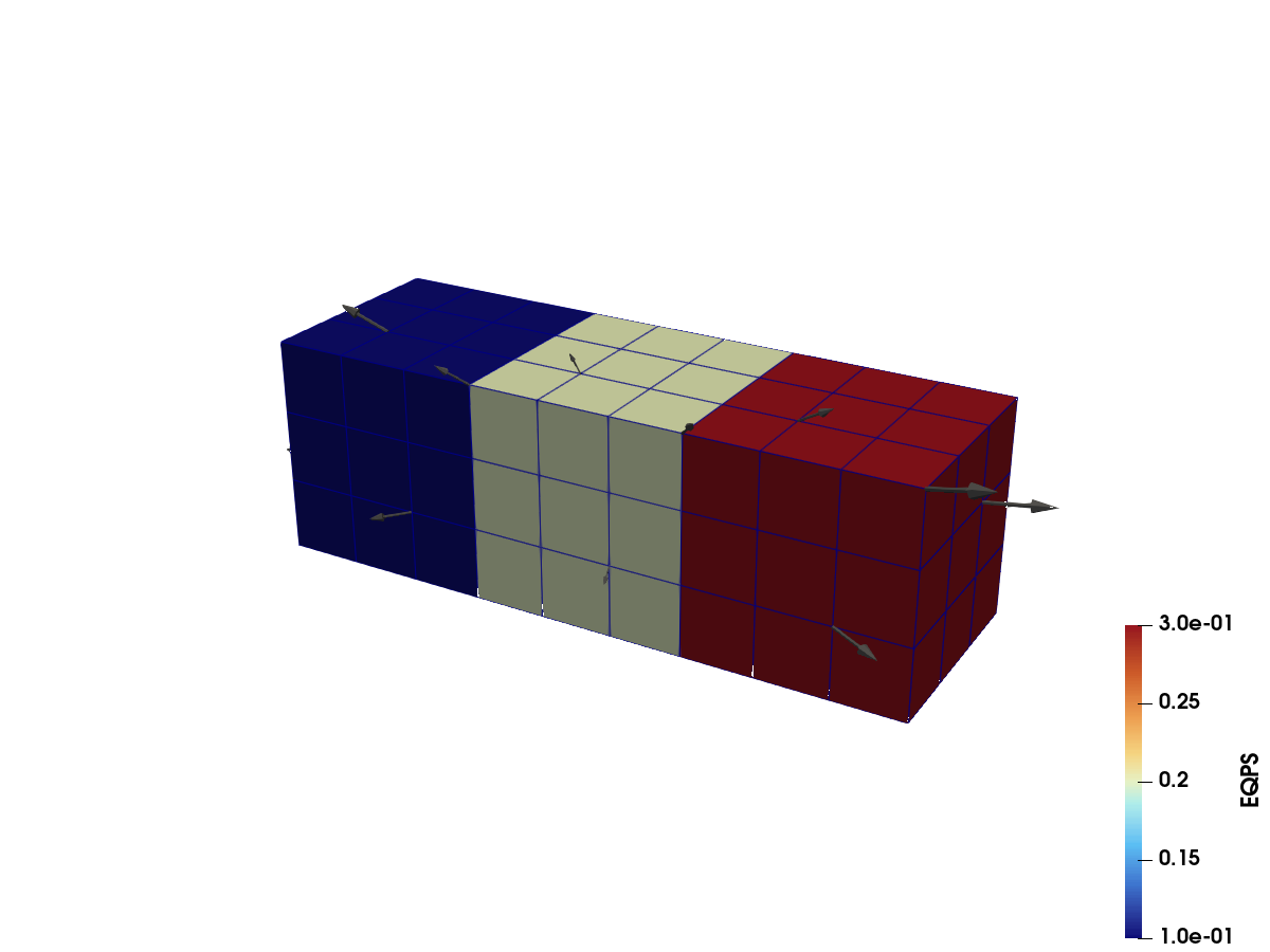
Port of the can-pvtu.vtkhdf example from the VTKHDF specification: an UnstructuredGrid written as three partitions, as a three-rank MPI simulation would produce. Each partition carries point and cell data, and the file also holds a global FieldData array. All partitions land in one file; VTK reads them back as a partitioned dataset.

What you'll learn: how to append partitions with local geometry and data, then recover their global ranges when reading.

The three partitions colored by EQPS, with a few VEL arrow glyphs:

using VTKHDF

A block of n³ hexahedra filling a unit cube at origin:

function hex_block(origin; n = 3)
    corners = vec(collect(Iterators.product(0:n, 0:n, 0:n)))
    points = [origin[d] + c[d] / n for d in 1:3, c in corners]
    id(i, j, k) = i + 1 + (n + 1) * (j + (n + 1) * k)
    cells = vec(
        [
            MeshCell(
                    VTKCellTypes.VTK_HEXAHEDRON, [
                        id(i, j, k), id(i + 1, j, k), id(i + 1, j + 1, k), id(i, j + 1, k),
                        id(i, j, k + 1), id(i + 1, j, k + 1), id(i + 1, j + 1, k + 1), id(i, j + 1, k + 1),
                    ]
                )
                for i in 0:(n - 1), j in 0:(n - 1), k in 0:(n - 1)
        ]
    )
    return points, cells
end

Creating the file with the VTKUnstructuredGrid() tag defers the geometry; partitions are then appended one by one together with their data.

vtk = vtkhdf_grid(VTKUnstructuredGrid(), "can")
for (partition_id, origin) in enumerate(((0, 0, 0), (1, 0, 0), (2, 0, 0)))
    points, cells = hex_block(origin)
    velocity = points .- [1.5, 0.5, 0.5]
    add_partition(
        vtk, points, cells;
        pointdata = ("VEL" => velocity,),
        celldata = ("EQPS" => fill(0.1 * partition_id, length(cells)),),
    )
end
vtk["TimeValue", VTKFieldData()] = [0.001]
close(vtk)

Reading it back

The same file can be opened again with vtkhdf_open:

r = vtkhdf_open("can")

VTKHDFReader{ReadUnstructured} (open)

Geometry comes back through read_points/read_cells. The partitions are concatenated and the cell connectivity is renumbered to match, so the cells index directly into the returned points.

Each partition contributes 4³ = 64 points and 3³ = 27 cells, so the combined reader exposes 192 points and 81 cells:

size(read_points(r)), length(read_cells(r)) # ((3, 192), 81)

((3, 192), 81)

Data arrays use the same indexing syntax as writing, and the partition structure is recoverable as index ranges into them:

The three constant partition values span 0.1 through 0.3:

extrema(r["EQPS", VTKCellData()]) # (0.1, 0.3)

(0.1, 0.30000000000000004)

These ranges show which 27-cell slice came from each partition:

VTKHDF.partition_ranges(r).cells # [1:27, 28:54, 55:81]

3-element Vector{UnitRange{Int64}}:
 1:27
 28:54
 55:81

close(r)