Boundary and initial conditions

Every PDE is accompanied with boundary conditions. There are different types of boundary conditions, and they need to be handled in different ways. Below we discuss how to handle the most common ones, Dirichlet, Neumann, and Robin boundary conditions, and how to do it in Ferrite.

While boundary conditions can be applied directly to nodes, vertices, edges, or faces, they are most commonly applied to facets. Each facet is described by a FacetIndex. When adding boundary conditions to points instead, vertices are preferred over nodes.

• Dirichlet boundary conditions
• Neumann boundary conditions
• Robin boundary conditions
• Periodic boundary conditions
• Initial conditions

Dirichlet boundary conditions

At a Dirichlet boundary the unknown field is prescribed to a given value. For the discrete FE-solution this means that there are some degrees of freedom that are fixed. To handle Dirichlet boundary conditions in Ferrite we use the ConstraintHandler. A constraint handler is created from a DoF handler:

ch = ConstraintHandler(dh)

We can now create Dirichlet constraints and add them to the constraint handler. To create a Dirichlet constraint we need to specify a field name, a part of the boundary, and a function for computing the prescribed value. Example:

dbc1 = Dirichlet(    :u,                        # Name of the field    getfacetset(grid, "left"), # Part of the boundary    x -> 1.0,                  # Function mapping coordinate to a prescribed value)

The field name is given as a symbol, just like when the field was added to the dof handler, the part of the boundary where this constraint is active is given as a facet set, and the function computing the prescribed value should be of the form f(x) or f(x, t) (coordinate x and time t) and return the prescribed value(s).

left_right = union(getfacetset(grid, "left"), getfacetset(grid, "right"))

By default the constraint is added to all components of the given field. To add the constraint to selected components a fourth argument with the components should be passed to the constructor. Here is an example where a constraint is added to component 1 and 3 of a vector field :v:

dbc2 = Dirichlet(    :v,                        # Name of the field    getfacetset(grid, "left"), # Part of the boundary    x -> [0.0, 0.0],           # Function mapping coordinate to prescribed values    [1, 3],                    # Components)

Note that the return value of the function must match with the components – in the example above we prescribe components 1 and 3 to 0 so we return a vector of length 2.

Adding the constraints to the constraint handler is done with add!:

add!(ch, dbc1)add!(ch, dbc2)

Finally, just like for the dof handler, we need to use close! to finalize the constraint handler. Internally this will then compute the degrees-of-freedom that match the constraints we added.

close!(ch)

If one or more of the constraints depend on time, i.e. they are specified as f(x, t), the prescribed values can be recomputed in each new time step by calling update! with the proper time, e.g.:

for t in 0.0:0.1:1.0    update!(ch, t) # Compute prescribed values for this t    # Solve for time t...end

Projected Dirichlet boundary conditions

Some interpolations don't have nodal support points: $H(\mathrm{curl})$ interpolations, e.g., Nedelec, are associated to edges and faces, while $H(\mathrm{div})$ interpolations, e.g. RaviartThomas, are associated to facets. While normal Dirichlet boundary conditions assume the existence of such nodal support points, Ferrite provides the ProjectedDirichlet, which instead finds the degree of freedom values that minimizes the L2-distance between the prescribed function, $f(\boldsymbol{x},t,\boldsymbol{n})$, and the finite element interpolation space, cf. [9]. Although standard interpolations are not currently supported, the figure below illustrates well the difference between applying a standard Dirichlet condition and a ProjectedDirichlet condition when the prescribed function cannot be described by the chosen FE-interpolation.

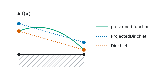
Here, we note that while the Dirichlet condition gives the correct value at the nodes, the ProjectedDirichlet gives a more accurate average boundary value (specifically the L2 projection of f(x) onto the finite element space).

Neumann boundary conditions

At the Neumann part of the boundary we know something about the gradient of the solution. Two different methods for applying these are described below. For complete examples that use Neumann boundary conditions, please see

• von-Mises-plasticity
• Hyperelasticity

Using the FacetIterator

A Neumann boundary contribution can be added by iterating over the relevant facetset by using the FacetIterator. For a scalar field, this can be done as

grid = generate_grid(Quadrilateral, (3, 3))dh = DofHandler(grid); add!(dh, :u, Lagrange{RefQuadrilateral, 1}()); close!(dh)fv = FacetValues(FacetQuadratureRule{RefQuadrilateral}(2), Lagrange{RefQuadrilateral, 1}())f = zeros(ndofs(dh))fe = zeros(ndofs_per_cell(dh))qn = 1.0    # Outward normal flux, q ⋅ n (heat leaving the domain)for fc in FacetIterator(dh, getfacetset(grid, "right"))    reinit!(fv, fc)    fill!(fe, 0)    for q_point in 1:getnquadpoints(fv)        dΓ = getdetJdV(fv, q_point)        for i in 1:getnbasefunctions(fv)            δu = shape_value(fv, q_point, i)            fe[i] -= δu * qn * dΓ        end    end    assemble!(f, celldofs(fc), fe)end

Alternatively, it is possible to add the values directly to the global f (without going through the local fe vector and then using assemble!):

for fc in FacetIterator(dh, getfacetset(grid, "right"))    reinit!(fv, fc)    dofs = celldofs(fc)    for q_point in 1:getnquadpoints(fv)        dΓ = getdetJdV(fv, q_point)        for i in 1:getnbasefunctions(fv)            δu = shape_value(fv, q_point, i)            f[dofs[i]] -= δu * qn * dΓ        end    endend

In the element routine

Alternatively, the boundary integral can be evaluated in the element routine, together with the contributions from the domain integrals:

function assemble_element!(Ke, fe, cell, facetvalues, ΓN, qn)    # ... contributions from the domain integrals to Ke and fe ...    # Contributions from the Neumann boundary    for facet in 1:nfacets(cell)        if (cellid(cell), facet) ∈ ΓN            reinit!(facetvalues, cell, facet)            for q_point in 1:getnquadpoints(facetvalues)                dΓ = getdetJdV(facetvalues, q_point)                for i in 1:getnbasefunctions(facetvalues)                    δu = shape_value(facetvalues, q_point, i)                    fe[i] -= δu * qn * dΓ                end            end        end    end    returnend

In the element routine we loop over all the facets of the cell, and check if this particular facet is located on the Neumann boundary, given by the facetset ΓN. If we have determined that the current facet is indeed on the boundary and in our facetset, then we reinitialize FacetValues for this facet, using reinit!. When reinit!ing FacetValues we also need to give the facet number in addition to the cell. Next we simply loop over the quadrature points of the facet, and then loop over all the test functions and add the contribution to the element force vector.

The element routine is then called in the loop over the cells, where the facetset is fetched from the grid once before the loop:

ΓN = getfacetset(grid, "Neumann Boundary")for cell in CellIterator(dh)    fill!(Ke, 0)    fill!(fe, 0)    assemble_element!(Ke, fe, cell, facetvalues, ΓN, qn)    assemble!(assembler, celldofs(cell), Ke, fe)end

Robin boundary conditions

At a Robin boundary a linear combination of the unknown field and its normal flux is prescribed. Consider, for example, the heat equation

\[\begin{aligned} \boldsymbol{\nabla} \cdot \boldsymbol{q} &= f \quad &\forall\, \boldsymbol{x} \in \Omega, \\ u &= g_\mathrm{D} \quad &\forall\, \boldsymbol{x} \in \Gamma_\mathrm{D}, \\ a\, u + b\, q_\mathrm{n} &= g_\mathrm{R} \quad &\forall\, \boldsymbol{x} \in \Gamma_\mathrm{R}, \end{aligned}\]

where $u$ is the temperature, $\boldsymbol{q} = -k \boldsymbol{\nabla} u$ the heat flux, $q_\mathrm{n} := \boldsymbol{q} \cdot \boldsymbol{n}$ the outward normal flux, and $a$, $b$ and $g_\mathrm{R}$ are given. For simplicity the boundary is split into a Dirichlet and a Robin part, $\Gamma = \Gamma_\mathrm{D} \cup \Gamma_\mathrm{R}$. Dirichlet ($b = 0$) and Neumann ($a = 0$) boundary conditions are special cases. Unlike Dirichlet boundary conditions, Robin boundary conditions are not imposed with the ConstraintHandler. Instead they are added weakly, as boundary integrals, just like Neumann boundary conditions.

Multiplying with a test function $\delta u$, integrating over the domain, and using partial integration gives

\[\int_\Omega k\, \boldsymbol{\nabla} \delta u \cdot \boldsymbol{\nabla} u\, \mathrm{d}\Omega + \int_{\Gamma_\mathrm{R}} \delta u\, q_\mathrm{n}\, \mathrm{d}\Gamma = \int_\Omega \delta u\, f\, \mathrm{d}\Omega,\]

where the test function vanishes on $\Gamma_\mathrm{D}$. Inserting $q_\mathrm{n} = (g_\mathrm{R} - a\, u) / b$ from the Robin boundary condition we obtain the weak form: Find $u \in \mathbb{U}$ s.t.

\[\int_\Omega k\, \boldsymbol{\nabla} \delta u \cdot \boldsymbol{\nabla} u\, \mathrm{d}\Omega - \int_{\Gamma_\mathrm{R}} \delta u\, \frac{a}{b}\, u\, \mathrm{d}\Gamma = \int_\Omega \delta u\, f\, \mathrm{d}\Omega - \int_{\Gamma_\mathrm{R}} \delta u\, \frac{g_\mathrm{R}}{b}\, \mathrm{d}\Gamma \quad \forall\, \delta u \in \mathbb{U}^0.\]

Compared to a Neumann boundary condition, which only contributes to the right hand side, the Robin boundary condition also contributes to the left hand side, since the boundary integral depends on the unknown $u$. After discretization this gives the contributions

\[K_{ij} \mathrel{+}= -\int_{\Gamma_\mathrm{R}} \phi_i\, \frac{a}{b}\, \phi_j\, \mathrm{d}\Gamma, \quad f_i \mathrel{+}= -\int_{\Gamma_\mathrm{R}} \phi_i\, \frac{g_\mathrm{R}}{b}\, \mathrm{d}\Gamma\]

to the stiffness matrix and the right hand side, respectively.

A common way to write the Robin boundary condition for heat transfer is

\[q_\mathrm{n} = k_\Gamma\, (u - u_\Gamma),\]

where $k_\Gamma$ is the heat transfer coefficient and $u_\Gamma$ the ambient temperature, i.e. heat flows out of the domain when it is warmer than its surroundings. This corresponds to $a = -k_\Gamma$, $b = 1$, and $g_\mathrm{R} = -k_\Gamma u_\Gamma$, and the weak form becomes

\[\int_\Omega k\, \boldsymbol{\nabla} \delta u \cdot \boldsymbol{\nabla} u\, \mathrm{d}\Omega + \int_{\Gamma_\mathrm{R}} \delta u\, k_\Gamma\, u\, \mathrm{d}\Gamma = \int_\Omega \delta u\, f\, \mathrm{d}\Omega + \int_{\Gamma_\mathrm{R}} \delta u\, k_\Gamma\, u_\Gamma\, \mathrm{d}\Gamma.\]

For the problem to be well-posed we need $k_\Gamma \geq 0$ ($a / b \leq 0$ in the general form).

The Robin contributions can be computed by iterating over the Robin part of the boundary with the FacetIterator, similar to Neumann boundary conditions. Since they contribute to both the stiffness matrix and the right hand side, we assemble them with an assembler. Here we assume that K and f already contain the contributions from the domain integrals, so we pass fillzero = false to start_assemble to keep them:

fv = FacetValues(FacetQuadratureRule{RefQuadrilateral}(2), Lagrange{RefQuadrilateral, 1}())kΓ = 2.0    # Heat transfer coefficientuΓ = 1.0    # Ambient temperatureKe = zeros(ndofs_per_cell(dh), ndofs_per_cell(dh))fe = zeros(ndofs_per_cell(dh))assembler = start_assemble(K, f; fillzero = false)for fc in FacetIterator(dh, getfacetset(grid, "right"))    reinit!(fv, fc)    fill!(Ke, 0)    fill!(fe, 0)    for q_point in 1:getnquadpoints(fv)        dΓ = getdetJdV(fv, q_point)        for i in 1:getnbasefunctions(fv)            δu = shape_value(fv, q_point, i)            fe[i] += δu * kΓ * uΓ * dΓ            for j in 1:getnbasefunctions(fv)                u = shape_value(fv, q_point, j)                Ke[i, j] += δu * kΓ * u * dΓ            end        end    end    assemble!(assembler, celldofs(fc), Ke, fe)end

If $k_\Gamma$ or $u_\Gamma$ vary along the boundary, they can be evaluated at the quadrature point coordinate, given by spatial_coordinate(fv, q_point, getcoordinates(fc)). As for Neumann boundary conditions, the contributions can also be computed in the element routine instead, by adding the facet loop to the computation of Ke and fe for each cell.

Periodic boundary conditions

Periodic boundary conditions ensure that the solution is periodic across two boundaries. To define the periodicity we first define the image boundary $\Gamma^+$ and the mirror boundary $\Gamma^-$. We also define a (unique) coordinate mapping between the image and the mirror: $\varphi:\ \Gamma^+\, \rightarrow\, \Gamma^-$. With the mapping we can, for every coordinate on the image, compute the corresponding coordinate on the mirror:

\[\boldsymbol{x}^- = \varphi(\boldsymbol{x}^+),\quad \boldsymbol{x}^- \in \Gamma^-,\, \boldsymbol{x}^+ \in \Gamma^+.\]

We now want to ensure that the solution on the image $\Gamma^+$ is mirrored on the mirror $\Gamma^-$. This periodicity constraint can thus be described by

\[u(\boldsymbol{x}^-) = u(\boldsymbol{x}^+).\]

Sometimes this is written as

\[\llbracket u \rrbracket = 0,\]

where $\llbracket \bullet \rrbracket := \bullet(\boldsymbol{x}^+) - \bullet(\boldsymbol{x}^-)$ is the "jump operator". Thus, this condition ensures that the jump, or difference, in the solution between the image and mirror boundary is zero – the solution becomes periodic. For a vector valued problem the periodicity constraint can in general be written as

\[\boldsymbol{u}(\boldsymbol{x}^-) = \boldsymbol{R} \cdot \boldsymbol{u}(\boldsymbol{x}^+) \quad \Leftrightarrow \quad \llbracket \boldsymbol{u} \rrbracket = \boldsymbol{R} \cdot \boldsymbol{u}(\boldsymbol{x}^+) - \boldsymbol{u}(\boldsymbol{x}^-) = \boldsymbol{0}\]

where $\boldsymbol{R}$ is a rotation matrix. If the mapping between mirror and image is simply a translation (e.g. sides of a cube) this matrix will be the identity matrix.

In Ferrite this type of periodic Dirichlet boundary conditions can be added to the ConstraintHandler by constructing an instance of PeriodicDirichlet. This is usually done it two steps. First we compute the mapping between mirror and image facets using collect_periodic_facets. Here we specify the mirror set and image sets (the sets are usually known or can be constructed easily ) and the mapping $\varphi$. Second we construct the constraint using the PeriodicDirichlet constructor. Here we specify which components of the function that should be constrained, and the rotation matrix $\boldsymbol{R}$ (when needed). When adding the constraint to the ConstraintHandler the resulting dof-mapping is computed.

Here is a simple example where periodicity is enforced for components 1 and 2 of the field :u between the mirror boundary set "left" and the image boundary set "right". Note that no rotation matrix is needed here since the mirror and image are parallel, just shifted in the $x$-direction (as seen by the mapping φ):

# Create a constraint handler from the dof handlerch = ConstraintHandler(dofhandler)# Compute the facet mappingφ(x) = x - Vec{2}((1.0, 0.0))facet_mapping = collect_periodic_facets(grid, "left", "right", φ)# Construct the periodic constraint for field :updbc = PeriodicDirichlet(:u, facet_mapping, [1, 2])# Add the constraint to the constraint handleradd!(ch, pdbc)# If no more constraints should be added we can closeclose!(ch)

Heterogeneous "periodic" constraint

It is also possible to define constraints of the form

\[\llbracket u \rrbracket = \llbracket f \rrbracket \quad \Leftrightarrow \quad u(\boldsymbol{x}^+) - u(\boldsymbol{x}^-) = f(\boldsymbol{x}^+) - f(\boldsymbol{x}^-),\]

where $f$ is a prescribed function. Although the constraint in this case is not technically periodic, PeriodicDirichlet can be used for this too. This is done by passing a function to PeriodicDirichlet, similar to Dirichlet, which, given the coordinate $\boldsymbol{x}$ and time t, computes the prescribed values of $f$ on the boundary.

Here is an example of how to implement this type of boundary condition, for a known function f:

pdbc = PeriodicDirichlet(    :u,    facet_mapping,    (x, t) -> f(x),    [1, 2],)

pdbc = PeriodicDirichlet(    :u,    facet_mapping,    (x, t) -> ū + ∇ū  ⋅ (x - x̄))

Initial conditions

When solving time-dependent problems, initial conditions, different from zero, may be required. For finite element formulations of ODE-type, i.e. $\boldsymbol{u}'(t) = \boldsymbol{f}(\boldsymbol{u}(t),t)$, where $\boldsymbol{u}(t)$ are the degrees of freedom, initial conditions can be specified by the apply_analytical! function. For example, specify the initial pressure as a function of the y-coordinate

ρ = 1000; g = 9.81    # density [kg/m³] and gravity [N/kg]grid = generate_grid(Quadrilateral, (10, 10))dh = DofHandler(grid); add!(dh, :u, Lagrange{RefQuadrilateral, 1}()^2); add!(dh, :p, Lagrange{RefQuadrilateral, 1}()); close!(dh)u = zeros(ndofs(dh))apply_analytical!(u, dh, :p, x -> ρ * g * x[2])

See also Transient heat equation for one example.